125. Competitive Equilibria with Arrow Securities#
125.1. Overview#
This lecture presents Python code for experimenting with competitive equilibria of an infinite-horizon pure exchange economy with
heterogeneous agents,
endowments of a single consumption good that are person-specific functions of a common Markov state,
complete markets in one-period Arrow state-contingent securities,
discounted expected utility preferences of a kind often used in macroeconomics and finance,
identical preferences across agents, with a common discount factor and a constant relative risk aversion (CRRA) one-period utility function, and
common beliefs among agents.
Differences in their endowments make individuals want to reallocate consumption goods across time and Markov states.
Identical CRRA preferences imply that equilibrium consumption shares are constant, so we can compute equilibrium prices from the aggregate endowment before we compute the equilibrium distribution of wealth.
We impose restrictions that allow us to Bellmanize competitive equilibrium prices and quantities.
We use Bellman equations to describe
asset prices,
continuation wealth levels for each person, and
state-by-state natural debt limits for each person.
In the course of presenting the model we shall encounter these important ideas:
a resolvent operator widely used in this class of models,
the absence of borrowing limits in finite-horizon economies,
state-by-state borrowing limits required in infinite-horizon economies,
a counterpart of the law of iterated expectations known as a law of iterated values, and
a state variable degeneracy that prevails within a competitive equilibrium and that opens the way to various appearances of resolvent operators.
The lecture implements a Python version of the model presented in section 9.3.3 of [Ljungqvist and Sargent, 2018].
Readers will find it helpful to know the finite-state Markov asset pricing formulas of Asset Pricing: Finite State Models and the Markov chain concepts of Finite Markov Chains.
Let’s start with some imports.
import numpy as np
import matplotlib.pyplot as plt

np.set_printoptions(suppress=True)
125.2. The setting#
125.2.1. Preferences and endowments#
In each period \(t \geq 0\), a stochastic event \(s_t \in \mathbf{S}\) is realized.
Let the history of events up until time \(t\) be denoted \(s^t = [s_0, s_1, \ldots, s_{t-1}, s_t]\).
The unconditional probability of observing a particular sequence of events \(s^t\) is given by a probability measure \(\pi_t(s^t)\).
For \(t > \tau\), we write the probability of observing \(s^t\) conditional on the realization of \(s^\tau\) as \(\pi_t(s^t \mid s^\tau)\).
We assume that trading occurs after observing \(s_0\), which we capture by setting \(\pi_0(s_0) = 1\) for the initially given value of \(s_0\).
In this lecture we follow much of macroeconomics and econometrics and assume that \(\pi_t(s^t)\) is induced by a Markov process.
There are \(K\) consumers named \(k = 1, \ldots, K\).
Consumer \(k\) owns a stochastic endowment of one good \(y_t^k(s^t)\) that depends on the history \(s^t\).
The history \(s^t\) is publicly observable.
Consumer \(k\) purchases a history-dependent consumption plan \(c^k = \{c_t^k(s^t)\}_{t=0}^\infty\).
All consumers order consumption plans by
where \(0 < \beta < 1\).
The right side equals \(E_0 \sum_{t=0}^\infty \beta^t u(c_t^k)\), where \(E_0\) is the mathematical expectation operator conditioned on \(s_0\).
Here \(u(c)\) is an increasing, twice continuously differentiable, strictly concave function of consumption \(c \geq 0\) of one good.
The utility function satisfies the Inada condition
This condition implies that each agent chooses strictly positive consumption for every date-history pair \((t, s^t)\) whenever the present value of its endowment is positive.
Those interior solutions allow us to confine our analysis to Euler equations that hold with equality, and they guarantee that natural debt limits don’t bind in economies like ours with sequential trading of Arrow securities.
We adopt the assumption, routinely employed in much of macroeconomics, that consumers share probabilities \(\pi_t(s^t)\) for all \(t\) and \(s^t\).
A feasible allocation satisfies
for all \(t\) and for all \(s^t\).
Until we reach the section on computing an equilibrium, \(u\) need only satisfy the properties listed above.
From then on we specialize to CRRA utility.
125.3. Markov asset prices#
Before setting up the equilibrium, we summarize formulas for computing asset prices in a Markov setting.
These formulas are developed at greater length in Asset Pricing: Finite State Models.
The setup assumes the following infrastructure:
Markov states \(s \in \mathbf{S} = \{\bar{s}_1, \ldots, \bar{s}_n\}\) governed by an \(n\)-state Markov chain with transition probability
a collection \(h = 1, \ldots, H\) of assets, where asset \(h\) pays \(d^h(s)\) in state \(s\), so that \(d^h\) is an \(n \times 1\) vector; and
an \(n \times n\) pricing kernel \(Q\) for one-period Arrow securities, where \(Q_{ij}\) is the price at time \(t\) in state \(s_t = \bar s_i\) of one unit of consumption delivered at time \(t+1\) if \(s_{t+1} = \bar s_j\).
The price in state \(\bar s_i\) of a one-period risk-free bond that pays one unit of consumption in every state is \(\sum_j Q_{ij}\).
The gross rate of return on that bond is therefore
125.3.1. An exogenous pricing kernel#
For now we take the pricing kernel \(Q\) as exogenous, that is, determined outside the model.
Two examples are
\(Q = \beta P\), where \(\beta \in (0, 1)\), and
\(Q_{ij} = m_{ij} P_{ij}\), where \(m_{ij} > 0\) is the value of a stochastic discount factor when the Markov state moves from \(\bar s_i\) to \(\bar s_j\).
The second example multiplies \(P\) element by element, not as a matrix product.
We now describe the prices of two types of assets.
The first is a cum-dividend stock that entitles its owner to the time \(t\) dividend and to the option to sell the asset at time \(t+1\).
Its price satisfies \(p^h(\bar s_i) = d^h(\bar s_i) + \sum_j Q_{ij} p^h(\bar s_j)\), so the vector \(p^h\) satisfies \(p^h = d^h + Q p^h\).
Provided every eigenvalue of \(Q\) has modulus less than one, this implies
The second is an ex-dividend stock purchased at the end of time \(t\), which entitles its owner to the time \(t+1\) dividend and to the option to sell the stock at time \(t+1\).
Its price is
Note
The matrix geometric sum \((I - Q)^{-1} = I + Q + Q^2 + \cdots\) is an example of a resolvent operator.
It converges when the spectral radius of \(Q\) is less than one.
Below we describe an equilibrium model with trading of one-period Arrow securities in which the pricing kernel is endogenous.
In constructing that model, we’ll repeatedly encounter formulas that remind us of these asset pricing formulas.
125.3.2. Multi-step transition probabilities and pricing kernels#
The \((i,j)\) component of the \(j\)-step-ahead transition matrix \(P^j\) is
To keep the notation light below, we write \(P_j(s_{t+j} \mid s_t)\) for these \(j\)-step transition probabilities, so that \(P_j\) is represented by the matrix \(P^j\).
In the same way, the price at time \(t\) in state \(s_t\) of one unit of consumption delivered at time \(t+j\) in state \(s_{t+j}\) is \(Q_j(s_{t+j} \mid s_t)\), represented by the matrix \(Q^j\).
We’ll use these objects to state a useful property of asset pricing theory.
125.3.3. Laws of iterated expectations and iterated values#
A law of iterated values has a mathematical structure that parallels a law of iterated expectations.
We can describe its structure readily in the Markov setting of this lecture.
Recall the following recursion satisfied by \(j\)-step-ahead transition probabilities for our finite-state Markov chain:
We can use this recursion to verify the law of iterated expectations applied to the conditional expectation of a random variable \(d(s_{t+j})\) conditioned on \(s_t\):
The pricing kernel for \(j\)-step-ahead Arrow securities satisfies the recursion
The time \(t\) value in Markov state \(s_t\) of a time \(t+j\) payout \(d(s_{t+j})\) is
The law of iterated values states that
We verify it with a string of equalities that are counterparts to those we used to verify the law of iterated expectations:
125.4. Recursive formulation#
Following section 9.3.3 of [Ljungqvist and Sargent, 2018], we now set up a competitive equilibrium of a pure exchange economy with complete markets in one-period Arrow securities.
When endowments \(y^k(s)\) are all functions of a common Markov state \(s\), the pricing kernel takes the form \(Q(s' \mid s)\), the price of one unit of consumption in state \(s'\) at date \(t+1\) when the Markov state at date \(t\) is \(s\).
This lets us formulate a consumer’s optimization problem recursively.
Consumer \(k\)’s state at time \(t\) is its financial wealth \(a_t^k\) and the Markov state \(s_t\).
Let \(v^k(a, s)\) be the optimal value of consumer \(k\)’s problem starting from state \((a, s)\).
Thus \(v^k(a, s)\) is the maximum expected discounted utility that consumer \(k\) with current financial wealth \(a\) can attain in Markov state \(s\).
The optimal value function satisfies the Bellman equation
where the maximization is subject to the budget constraint
and the constraints
The second set of constraints is a collection of state-by-state debt limits.
The value function and decision rule that solve the Bellman equation depend on the pricing kernel \(Q(\cdot \mid \cdot)\) because it appears in the budget constraint.
The first-order conditions for the problem on the right of the Bellman equation, together with a Benveniste–Scheinkman formula, imply
where it is understood that \(c_t^k = c^k(s_t)\) and \(c_{t+1}^k = c^k(s_{t+1})\).
125.4.1. Recursive competitive equilibrium#
A recursive competitive equilibrium is an initial distribution of wealth \(\vec a_0\), a set of borrowing limits \(\{\bar A^k(s)\}_{k=1}^K\), a pricing kernel \(Q(s' \mid s)\), sets of value functions \(\{v^k(a, s)\}_{k=1}^K\), and decision rules \(\{c^k(s), \hat a^k(s)\}_{k=1}^K\) such that
the state-by-state borrowing limits satisfy the recursion
for all \(k\), given \(a_0^k\), \(\bar A^k(s)\), and the pricing kernel, the value functions and decision rules solve the consumers’ problems;
for all realizations of \(\{s_t\}_{t=0}^\infty\), the consumption and asset portfolios \(\{\{c_t^k, \{\hat a_{t+1}^k(s')\}_{s'}\}_k\}_t\) satisfy \(\sum_k c_t^k = \sum_k y^k(s_t)\) and \(\sum_k \hat a_{t+1}^k(s') = 0\) for all \(t\) and \(s'\); and
the initial financial wealth vector \(\vec a_0\) satisfies \(\sum_{k=1}^K a_0^k = 0\).
The third condition asserts that goods markets clear and that there are zero net aggregate claims in all Markov states.
The fourth condition asserts that the economy is closed and starts from a situation in which there are zero net aggregate claims.
125.5. State variable degeneracy#
[Ljungqvist and Sargent, 2018] and Cass-Koopmans Competitive Equilibrium describe a different timing protocol, in which there is a complete menu of history-contingent claims on consumption at all dates and all trades occur once and for all at time \(0\).
For the allocation and pricing kernel of a recursive competitive equilibrium to coincide with those of that time \(0\) arrangement, we must impose \(a_0^k = 0\) for \(k = 1, \ldots, K\).
That initial condition ensures that at time \(0\) the present value of each consumer’s consumption equals the present value of its endowment stream, which is the single budget constraint of the time \(0\) arrangement.
Starting the system with \(a_0^k = 0\) for all \(k\) has a striking implication that we call state variable degeneracy.
Although two state variables \(a\) and \(s\) appear in the value function \(v^k(a, s)\), within a recursive competitive equilibrium that starts from \(a_0^k = 0\) for all \(k\) at initial Markov state \(s_0\), two outcomes prevail:
financial wealth \(a_t^k\) is an exact function of the Markov state \(s_t\), which we compute below, and
\(a_t^k = 0\) for all \(k\) whenever the Markov state \(s_t\) returns to \(s_0\).
The first finding asserts that within a competitive equilibrium the exogenous Markov state is all we require to track an individual, because financial wealth is redundant.
The second finding asserts that each household returns to the zero financial wealth with which it began life whenever the Markov state returns to its initial value.
That happens infinitely often if \(s_0\) is a recurrent state of the Markov chain, but it need not happen at all if \(s_0\) is transient; see Finite Markov Chains.
This outcome depends critically on there being complete markets in Arrow securities.
For example, it does not prevail in the incomplete markets setting of The Aiyagari Model, where a household’s wealth depends on its whole history of shocks.
125.6. Computing a competitive equilibrium#
Now we are ready to do some fun calculations.
We find it useful to think in terms of analytical inputs into and outputs from our general equilibrium theorizing.
125.6.1. Inputs and outputs#
The inputs are
Markov states \(s \in \mathbf{S} = \{\bar{s}_1, \ldots, \bar{s}_n\}\) governed by an \(n\)-state Markov chain with transition matrix \(P\);
\(K\) vectors of individual endowments \(y^k\), each of dimension \(n \times 1\) with components \(y^k(\bar s_i)\);
the \(n \times 1\) vector of aggregate endowments \(y(s) \equiv \sum_{k=1}^K y^k(s)\); and
preferences given by the common utility functional \(E_0 \sum_{t=0}^\infty \beta^t u(c_t^k)\) with discount factor \(\beta \in (0, 1)\) and CRRA one-period utility function
Feasibility requires
The outputs are
an \(n \times n\) pricing kernel \(Q\) for one-period Arrow securities;
the aggregate allocation, which in a pure exchange economy is \(c(s) = y(s)\);
a \(K \times 1\) distribution of wealth \(\alpha\) with \(\alpha_k \geq 0\) and \(\sum_{k=1}^K \alpha_k = 1\); and
\(K\) vectors of individual consumptions \(c^k\), each of dimension \(n \times 1\).
125.6.2. The pricing kernel#
For any agent \(k \in \{1, \ldots, K\}\), at the equilibrium allocation, the one-period Arrow securities pricing kernel satisfies
This follows from agent \(k\)’s first-order necessary conditions.
Because all agents face the same pricing kernel, the Euler equations of any two agents \(k\) and \(m\) imply
So the ratio \(c^k(s)/c^m(s)\) is the same in any two states connected by a positive transition probability, and hence in every state reachable from \(s_0\).
Consumption shares are therefore constant, and feasibility gives
for a distribution of wealth \(\alpha\) that satisfies \(\alpha_k \geq 0\) and \(\sum_{k=1}^K \alpha_k = 1\).
Note
Identical CRRA preferences also satisfy the conditions for Gorman aggregation, since Engel curves are linear with a common slope, so a representative consumer exists.
The constancy of consumption shares, however, follows directly from the Euler equations above.
This means that we can compute the pricing kernel from
This is the pricing kernel of the Lucas tree economy studied in Asset Pricing: Finite State Models, in which a representative consumer eats the aggregate endowment.
The pricing kernel \(Q\) does not depend on the vector \(\alpha\).
Key finding: We can compute competitive equilibrium prices prior to computing a distribution of wealth.
The wealth distribution \(\alpha\) is not arbitrary.
It is pinned down by the initial condition \(a_0^k = 0\), as we show below.
Formula (125.1) has a useful matrix form.
Let \(D = \mathrm{diag}\bigl(u'(y_1), \ldots, u'(y_n)\bigr)\).
Then \(Q = \beta D^{-1} P D\), so \(Q\) is similar to \(\beta P\).
Its eigenvalues are \(\beta\) times those of \(P\), and because \(P\) is a stochastic matrix, the spectral radius of \(Q\) equals \(\beta < 1\).
This guarantees that the resolvent \((I - Q)^{-1}\) used below exists.
The factorization is an instance of the transition independence structure exploited in The Recovery Theorem, a connection we pursue in Exercise 125.2.
125.6.3. Natural debt limits#
Having computed an equilibrium pricing kernel \(Q\), we can compute several values that are required to pose or represent the solution of an individual household’s optimization problem.
For each individual \(k\), let \(\bar A^k\) be the \(n \times 1\) vector with components \(\bar A^k(\bar s_i)\).
The recursion in the definition of equilibrium implies
In a competitive equilibrium of an infinite-horizon economy with sequential trading of one-period Arrow securities, \(\bar A^k(s)\) is a state-by-state limit on the quantity of one-period Arrow securities paying off in state \(s\) at time \(t+1\) that individual \(k\) can issue at time \(t\).
These are often called natural debt limits.
They equal the maximum amount that individual \(k\) can repay in state \(s\) even if it consumes nothing forevermore.
Note
If utility satisfies an Inada condition at zero consumption, or if consumption is simply required to be nonnegative, then a finite-horizon economy with sequential trading of one-period Arrow securities needs no natural debt limits.
See the section on a finite-horizon economy below.
125.6.4. Continuation wealth and optimal portfolios#
Continuation wealth plays an important role in Bellmanizing a competitive equilibrium with sequential trading of a complete set of one-period Arrow securities.
For each individual \(k\), let \(\psi^k\) be the \(n \times 1\) vector with components \(\psi^k(\bar s_i)\), the financial wealth that consumer \(k\) holds when the Markov state is \(\bar s_i\).
Continuation wealth satisfies
To see why, note that with consumption \(c^k = \alpha_k y\) and a portfolio \(\hat a^k(s') = \psi^k(s')\), the budget constraint holds with equality in every state exactly when \(\psi^k = \alpha_k y - y^k + Q \psi^k\).
Summing over \(k\) shows that \(\sum_{k=1}^K \psi^k = 0_{n \times 1}\), so Arrow security markets clear.
A nifty feature of the model is that an optimal portfolio of a type \(k\) agent equals the continuation wealth that we just computed.
Thus, agent \(k\)’s purchases of Arrow securities that pay off next period depend only on next period’s Markov state and equal
125.6.5. The equilibrium wealth distribution#
With the initial state being a particular state \(s_0 \in \{\bar{s}_1, \ldots, \bar{s}_n\}\), we must have
so that every agent starts debt-free and holding no financial assets.
This means that the equilibrium distribution of wealth satisfies
where \(V \equiv \left[I - Q\right]^{-1}\) and \(V_z\) is the row of \(V\) corresponding to the initial state \(s_0\).
Since \(\sum_{k=1}^K V_z y^k = V_z y\), we have \(\sum_{k=1}^K \alpha_k = 1\).
Comparing (125.5) with (125.2) gives a revealing interpretation,
Each consumer’s share of aggregate consumption equals its share of the value, in the initial state, of the aggregate endowment.
Because \(\alpha\) depends on \(s_0\) through \(V_z\), the same economy started in different Markov states delivers different wealth distributions.
125.6.6. Value functions#
We can also compute optimal value functions in a competitive equilibrium with trades in a complete set of one-period state-contingent Arrow securities.
Call the optimal value function of consumer \(k\) the \(n \times 1\) vector \(J^k\).
For the infinite-horizon economy now under study,
where \(u(\alpha_k y)\) is the \(n \times 1\) vector with components \(u(\alpha_k y_i)\).
125.6.7. Summary of the algorithm#
Here is the logical flow of an algorithm to compute a competitive equilibrium:
compute \(Q\) from the aggregate endowment using formula (125.1);
compute the distribution of wealth \(\alpha\) from formula (125.5);
using \(\alpha\), assign each consumer \(k\) the share \(\alpha_k\) of the aggregate endowment in each state;
compute continuation wealths from the \(\alpha\)-dependent formula (125.3);
set agent \(k\)’s portfolio equal to its continuation wealth state by state, as in (125.4); and
compute value functions \(J^k\).
125.7. Finite horizon#
We now describe a finite-horizon version of the economy that operates for \(T+1\) periods \(t \in \mathbf{T} = \{0, 1, \ldots, T\}\).
We’ll want time-dependent counterparts of the objects described above, with one important exception: we won’t need borrowing limits.
Borrowing limits aren’t required in a finite-horizon economy in which the one-period utility function \(u(c)\) satisfies an Inada condition that sends the marginal utility of consumption to infinity as consumption approaches zero.
Nonnegativity of consumption at all \(t \in \mathbf{T}\) automatically limits borrowing, because no one can end period \(T\) in debt.
For each individual \(k\) and date \(t\), let \(\psi_t^k\) be the \(n \times 1\) vector of continuation wealths.
At the terminal date there is no future to finance, so \(\psi_T^k = \alpha_k y - y^k\).
Working backward with the budget constraint \(\psi_t^k = \alpha_k y - y^k + Q \psi_{t+1}^k\) gives
As before, \(\sum_{k=1}^K \psi_t^k = 0_{n \times 1}\) for all \(t \in \mathbf{T}\).
With the initial state being a particular state \(s_0\), we must have
which means the equilibrium distribution of wealth satisfies
where now
and \(V_z\) is the row of \(V\) corresponding to the initial state \(s_0\).
Note
In the finite-horizon economy, continuation wealth depends on calendar time as well as on the Markov state.
The initial condition sets \(\psi_0^k(s_0) = 0\), but when the Markov state returns to \(s_0\) at a later date \(t\), fewer periods remain, the geometric sum in (125.6) is truncated sooner, and in general \(\psi_t^k(s_0) \neq 0\).
The strong form of state variable degeneracy, in which wealth is a function of the Markov state alone, is special to the infinite horizon.
Exercise 125.3 explores this.
To compute a competitive equilibrium with Arrow securities in the finite-horizon Markov economy,
compute \(Q\) from the aggregate endowment using formula (125.1);
compute the distribution of wealth \(\alpha\) from formulas (125.7) and (125.8);
using \(\alpha\), assign each consumer \(k\) the share \(\alpha_k\) of the aggregate endowment in each state;
compute continuation wealths from formula (125.6); and
set agent \(k\)’s portfolio equal to its continuation wealth state by state.
The value function of consumer \(k\) at time \(t\) is
125.8. Python code#
We now create a Python class to compute the objects that comprise a competitive equilibrium with sequential trading of one-period Arrow securities.
The class handles both infinite-horizon economies and finite-horizon economies indexed by horizon \(T\).
Every geometric sum in the lecture has the form \(I + M + \cdots\), with \(M = Q\) for prices and wealth and \(M = \beta P\) for values, so a single helper method computes them all.
In the finite-horizon case the helper works backward with the recursion \(S_t = I + M S_{t+1}\), starting from \(S_T = I\).
With \(M = Q\), this recursion is the law of iterated values at work: the time \(t\) value of payouts from \(t\) through \(T\) is the payout at \(t\) plus the time \(t\) value of the time \(t+1\) value of the remaining payouts.
With \(M = \beta P\), it is the law of iterated expectations applied to discounted utility.
The class also has a method that prices an asset with dividend vector \(d\) by applying these sums, which delivers the cum-dividend price \(p = d + Q d + Q^2 d + \cdots\) and the ex-dividend price \(p - d\).
In the finite-horizon case, arrays that depend on time are ordered from \(t = 0\) to \(t = T\), so that ψ[t] is \(\psi_t\) and J[t] is \(J_t\).
In the infinite-horizon case they have a single leading element.
class RecurCompetitive:
    """
    A competitive equilibrium with complete markets in one-period
    Arrow securities.

    Parameters
    ----------
    s : array of length n
        Markov states
    P : n x n array
        Markov transition matrix
    ys : n x K array
        endowments, with column k holding agent k's endowment
    γ : float
        coefficient of relative risk aversion
    β : float
        discount factor
    T : int or None
        time horizon, None for an infinite horizon
    """

    def __init__(self, s, P, ys, γ=0.5, β=0.98, T=None):

        self.s, self.P, self.ys = s, P, ys
        self.γ, self.β, self.T = γ, β, T
        self.n, self.K = ys.shape
        self.y = ys.sum(axis=1)                  # aggregate endowment

        self.Q = self.pricing_kernel()
        self.PRF = self.Q.sum(axis=1)            # price of a risk-free bond
        self.R = 1 / self.PRF                    # gross risk-free rate

        # V[t] = I + Q + ... + Q^(T-t), or [(I - Q)^(-1)] if T is None
        self.V = self.geometric_sums(self.Q)

        # time-0 values of endowments, the natural debt limits
        self.A = self.asset_price(ys)

    def u(self, c):
        "CRRA utility"
        return c ** (1 - self.γ) / (1 - self.γ)

    def u_prime(self, c):
        "Marginal utility"
        return c ** (-self.γ)

    def pricing_kernel(self):
        "Pricing kernel Q from equation (eq:Qformula)"
        mu = self.u_prime(self.y)
        return self.β * self.P * mu[None, :] / mu[:, None]

    def geometric_sums(self, M):
        """
        Return [(I - M)^(-1)] if T is None; otherwise return the sequence
        S[0], ..., S[T] with S[t] = I + M + ... + M^(T-t).
        """
        n, T = self.n, self.T
        if T is None:
            return np.linalg.inv(np.eye(n) - M)[None, :, :]
        S = np.empty((T+1, n, n))
        S[T] = np.eye(n)
        for t in range(T-1, -1, -1):
            S[t] = np.eye(n) + M @ S[t+1]      # law of iterated values
        return S

    def asset_price(self, d, ex_dividend=False):
        """
        Time-0 price of an asset with dividend vector d (n or n x K):
        cum-dividend p = d + Q d + Q^2 d + ..., or ex-dividend p - d.
        """
        p = self.V[0] @ d
        return p - d if ex_dividend else p

    def wealth_distribution(self, s0_idx):
        "Wealth distribution α when the initial state has index s0_idx"
        self.s0_idx = s0_idx
        V_z = self.V[0, s0_idx, :]
        self.α = V_z @ self.ys / (V_z @ self.y)
        return self.α

    def continuation_wealths(self):
        "Continuation wealths ψ, with ψ[t, i, k] = ψ_t^k(s_i)"
        excess = np.outer(self.y, self.α) - self.ys     # α_k y - y^k
        self.ψ = self.V @ excess
        return self.ψ

    def value_functions(self):
        "Value functions J, with J[t, i, k] = J_t^k(s_i)"
        flow = self.u(np.outer(self.y, self.α))         # u(α_k y)
        self.J = self.geometric_sums(self.β * self.P) @ flow
        return self.J
125.9. Examples#
We’ll use our code to construct equilibrium objects in several example economies.
Our first several examples are infinite-horizon economies.
Our final example is a finite-horizon economy.
Unless we say otherwise, examples use the default parameter values \(\gamma = 0.5\) and \(\beta = 0.98\).
125.9.1. Example 1: a constant aggregate endowment#
Two agents have perfectly negatively correlated endowments, so the aggregate endowment is constant.
s = np.array([0, 1])
P = np.array([[.5, .5],
              [.5, .5]])

ys = np.empty((2, 2))
ys[:, 0] = 1 - s       # agent 1
ys[:, 1] = s           # agent 2

ex1 = RecurCompetitive(s, P, ys)
print("aggregate endowment y =", ex1.y)
print("pricing kernel Q = \n", ex1.Q)
print("risk-free rate R =", ex1.R)
print("natural debt limits A = \n", ex1.A)
aggregate endowment y = [1. 1.]
pricing kernel Q =
 [[0.49 0.49]
 [0.49 0.49]]
risk-free rate R = [1.02040816 1.02040816]
natural debt limits A =
 [[25.5 24.5]
 [24.5 25.5]]
Because the aggregate endowment is constant, marginal utility is constant, so \(Q = \beta P\) and the risk-free rate is \(\beta^{-1}\) in both states.
# initial state is state 1
print(f'α = {ex1.wealth_distribution(s0_idx=0)}')
print(f'ψ = \n{ex1.continuation_wealths()}')
print(f'J = \n{ex1.value_functions()}')
print(f'share of natural debt limits in s0: {ex1.A[0] / ex1.A[0].sum()}')
α = [0.51 0.49]
ψ =
[[[-0.  0.]
  [ 1. -1.]]]
J =
[[[71.41428429 70.        ]
  [71.41428429 70.        ]]]
share of natural debt limits in s0: [0.51 0.49]
When the economy starts in state 1, agent 1 receives slightly more than half of aggregate consumption.
Its endowment arrives in the initial period, and consumption received sooner is discounted less.
As the last line confirms, each agent’s consumption share equals its share of the natural debt limits in the initial state.
In state 2, where agent 1 has no endowment, agent 1 holds financial wealth of one unit, which finances its consumption, and agent 2 owes exactly that amount.
# initial state is state 2
print(f'α = {ex1.wealth_distribution(s0_idx=1)}')
print(f'ψ = \n{ex1.continuation_wealths()}')
print(f'J = \n{ex1.value_functions()}')
α = [0.49 0.51]
ψ =
[[[-1.  1.]
  [ 0. -0.]]]
J =
[[[70.         71.41428429]
  [70.         71.41428429]]]
Starting in state 2 simply swaps the roles of the two agents.
125.9.2. Example 2: a fluctuating aggregate endowment#
Now agent 1 has a constant endowment while agent 2’s endowment fluctuates, so the aggregate endowment fluctuates.
s = np.array([1, 2])
P = np.array([[.5, .5],
              [.5, .5]])

ys = np.empty((2, 2))
ys[:, 0] = 1.5         # agent 1
ys[:, 1] = s           # agent 2

ex2 = RecurCompetitive(s, P, ys)

print("aggregate endowment y =", ex2.y)
print("pricing kernel Q = \n", ex2.Q)
print("risk-free rate R =", ex2.R)
print("natural debt limits A = \n", ex2.A)
aggregate endowment y = [2.5 3.5]
pricing kernel Q =
 [[0.49       0.41412558]
 [0.57977582 0.49      ]]
risk-free rate R = [1.10604104 0.93477529]
natural debt limits A =
 [[69.30941886 66.91255848]
 [81.73318641 79.98879094]]
The pricing kernels in examples 1 and 2 differ because the aggregate endowment is constant in example 1 but differs across states in example 2.
We can check two off-diagonal entries of \(Q\) directly against formula (125.1).
print(ex2.β * ex2.u_prime(3.5) / ex2.u_prime(2.5) * ex2.P[0, 1], ex2.Q[0, 1])
print(ex2.β * ex2.u_prime(2.5) / ex2.u_prime(3.5) * ex2.P[1, 0], ex2.Q[1, 0])
0.4141255848169731 0.4141255848169731
0.5797758187437624 0.5797758187437624
A claim to consumption in the high-endowment state is cheap, because marginal utility is low there.
The risk-free rate is high in the low-endowment state, where consumption is expected to rise, and low in the high-endowment state, where consumption is expected to fall.
Now let’s price some risky assets with the formulas \(p^h = (I - Q)^{-1} d^h\) and \(p^h = (I - Q)^{-1} Q d^h\) from the section on Markov asset prices.
We price a Lucas tree, which pays the aggregate endowment as its dividend, and claims to each agent’s endowment stream.
p_tree = ex2.asset_price(ex2.y)
p_tree_ex = ex2.asset_price(ex2.y, ex_dividend=True)

print("cum-dividend tree price     p =", p_tree)
print("ex-dividend tree price      p =", p_tree_ex)
print("price-dividend ratio (ex)     =", p_tree_ex / ex2.y)
print("Bellman residual |p - d - Qp| =",
      np.abs(p_tree - ex2.y - ex2.Q @ p_tree).max())
print("claims to endowments = \n", ex2.asset_price(ex2.ys))
cum-dividend tree price     p = [136.22197734 161.72197734]
ex-dividend tree price      p = [133.72197734 158.22197734]
price-dividend ratio (ex)     = [53.48879094 45.20627924]
Bellman residual |p - d - Qp| = 0.0
claims to endowments =
 [[69.30941886 66.91255848]
 [81.73318641 79.98879094]]
The cum-dividend price satisfies the one-step Bellman equation \(p = d + Q p\) to machine precision.
The ex-dividend price-dividend ratio is higher in the low-endowment state, where the current dividend is low relative to expected future dividends.
The last array reproduces the natural debt limits computed above: agent \(k\)’s natural debt limit in state \(s\) is the cum-dividend price of a claim to agent \(k\)’s own endowment stream.
That is why an agent can always repay a debt no larger than \(\bar A^k(s)\): it could sell the claim to its endowment and consume nothing forever.
# initial state is state 1
print(f'α = {ex2.wealth_distribution(s0_idx=0)}')
print(f'ψ = \n{ex2.continuation_wealths()}')
print(f'J = \n{ex2.value_functions()}')
α = [0.50879763 0.49120237]
ψ =
[[[ 0.          0.        ]
  [ 0.55057195 -0.55057195]]]
J =
[[[122.907875   120.76397493]
  [123.32114686 121.17003803]]]
# initial state is state 2
print(f'α = {ex2.wealth_distribution(s0_idx=1)}')
print(f'ψ = \n{ex2.continuation_wealths()}')
print(f'J = \n{ex2.value_functions()}')
α = [0.50539319 0.49460681]
ψ =
[[[-0.46375886  0.46375886]
  [-0.         -0.        ]]]
J =
[[[122.49598809 121.18174895]
  [122.907875   121.58921679]]]
125.9.3. Example 3: an absorbing state#
In this example state 2 is absorbing, so state 1 is transient.
s = np.array([1, 2])

λ = 0.9
P = np.array([[1-λ, λ],
              [0, 1]])

ys = np.empty((2, 2))
ys[:, 0] = [1, 0]      # agent 1
ys[:, 1] = [0, 1]      # agent 2

ex3 = RecurCompetitive(s, P, ys)

print("pricing kernel Q = \n", ex3.Q)
print("natural debt limits A = \n", ex3.A)
pricing kernel Q =
 [[0.098 0.882]
 [0.    0.98 ]]
natural debt limits A =
 [[ 1.10864745 48.89135255]
 [ 0.         50.        ]]
The natural debt limit for agent 1 in state 2 is \(0\).
Once the economy enters the absorbing state, agent 1 never receives another unit of endowment, so it cannot credibly promise to repay anything.
# initial state is state 1
print(f'α = {ex3.wealth_distribution(s0_idx=0)}')
print(f'ψ = \n{ex3.continuation_wealths()}')
print(f'J = \n{ex3.value_functions()}')
α = [0.02217295 0.97782705]
ψ =
[[[ 0.         -0.        ]
  [ 1.10864745 -1.10864745]]]
J =
[[[14.89058394 98.88513796]
  [14.89058394 98.88513796]]]
Starting in state 1, agent 1 receives only a small share of aggregate consumption, because its endowment arrives only while the economy remains in the transient state.
Because state 1 is transient, the economy eventually leaves it for good, and agents’ wealths do not recurrently return to zero.
# initial state is state 2
print(f'α = {ex3.wealth_distribution(s0_idx=1)}')
print(f'ψ = \n{ex3.continuation_wealths()}')
print(f'J = \n{ex3.value_functions()}')
α = [0. 1.]
ψ =
[[[-1.10864745  1.10864745]
  [ 0.          0.        ]]]
J =
[[[  0. 100.]
  [  0. 100.]]]
Starting in the absorbing state, agent 1 owns nothing of value, so \(\alpha_1 = 0\) and agent 1 consumes nothing forever.
This corner is consistent with the discussion of the Inada condition above, which guarantees interior consumption only for agents whose endowments have positive value.
For the specification of the Markov chain in example 3, let’s see how the equilibrium wealth distribution varies with the transition probability \(\lambda\).
λ_seq = np.linspace(0, 0.99, 100)

# prepare containers
αs0_seq = np.empty((len(λ_seq), 2))
αs1_seq = np.empty((len(λ_seq), 2))

for i, λ in enumerate(λ_seq):
    P_λ = np.array([[1-λ, λ],
                    [0, 1]])
    ex3_λ = RecurCompetitive(s, P_λ, ys)

    # initial state s0 = 1
    αs0_seq[i, :] = ex3_λ.wealth_distribution(s0_idx=0)

    # initial state s0 = 2
    αs1_seq[i, :] = ex3_λ.wealth_distribution(s0_idx=1)
fig, axs = plt.subplots(1, 2, figsize=(12, 4))

for i, αs_seq in enumerate([αs0_seq, αs1_seq]):
    for j in range(2):
        axs[i].plot(λ_seq, αs_seq[:, j], label=f'$\\alpha_{j+1}$')
    axs[i].set_xlabel(r'$\lambda$')
    axs[i].set_title(f'initial state $s_0 = {s[i]}$')
    axs[i].legend()

plt.show()
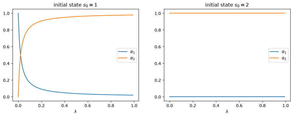
When the economy starts in state 1, a higher probability \(\lambda\) of leaving that state for good shortens the expected duration of agent 1’s endowment and lowers its wealth share.
When the economy starts in the absorbing state 2, \(\lambda\) is irrelevant and agent 2 owns everything.
125.9.4. Example 4: prosperity, a moderate state, and recession#
Our last infinite-horizon example has three Markov states, which we interpret as prosperity, a moderate state, and recession.
s = np.array([1, 2, 3])

λ = .9
μ = .9
δ = .05

# prosperous, moderate, and recession states
P = np.array([[1-λ, λ, 0],
              [(1-μ)/2, μ, (1-μ)/2],
              [(1-δ)/2, (1-δ)/2, δ]])

ys = np.empty((3, 2))
ys[:, 0] = [.25, .75, .2]      # agent 1
ys[:, 1] = [1.25, .25, .2]     # agent 2

ex4 = RecurCompetitive(s, P, ys)

print("rows of P sum to", P.sum(axis=1))
print("aggregate endowment y =", ex4.y)
print("pricing kernel Q = \n", ex4.Q)
print("risk-free rate R =", ex4.R)
print("natural debt limits A = \n", ex4.A)
rows of P sum to [1. 1. 1.]
aggregate endowment y = [1.5 1.  0.4]
pricing kernel Q =
 [[0.098      1.08022498 0.        ]
 [0.04000833 0.882      0.0774758 ]
 [0.24038317 0.29440805 0.049     ]]
risk-free rate R = [0.84873434 1.00051613 1.71294115]
natural debt limits A =
 [[41.66943407 19.83317897]
 [34.56301265 15.40376106]
 [21.44296495  9.99216994]]
The moderate state is highly persistent, and the economy moves out of recession quickly.
The gross risk-free rate is below one in prosperity, where aggregate consumption is expected to fall, and well above one in recession, where it is expected to recover.
for i in range(3):
    print(f"initial state is state {i+1}")
    print(f'α = {ex4.wealth_distribution(s0_idx=i)}')
    print(f'ψ = \n{ex4.continuation_wealths()}')
    print(f'J = \n{ex4.value_functions()}\n')
initial state is state 1
α = [0.67752299 0.32247701]
ψ =
[[[-0.         -0.        ]
  [-0.7093749   0.7093749 ]
  [-0.14493847  0.14493847]]]
J =
[[[82.66847975 57.03314431]
  [82.25708619 56.7493231 ]
  [81.82336679 56.45009924]]]

initial state is state 2
α = [0.69171992 0.30828008]
ψ =
[[[ 0.87314842 -0.87314842]
  [ 0.         -0.        ]
  [ 0.30134401 -0.30134401]]]
J =
[[[83.53011415 55.76358242]
  [83.11443273 55.48607909]
  [82.67619277 55.19351598]]]

initial state is state 3
α = [0.6821337 0.3178663]
ψ =
[[[ 0.28357106 -0.28357106]
  [-0.47899231  0.47899231]
  [-0.         -0.        ]]]
J =
[[[82.9492928  56.62395182]
  [82.53650179 56.34216692]
  [82.1013091  56.04508989]]]
Agent 1, whose endowment is concentrated in the persistent moderate state, receives about two thirds of aggregate consumption whichever state the economy starts in.
125.9.5. A finite-horizon example#
We now revisit the economy defined in example 1, but set the time horizon to \(T = 10\).
s = np.array([0, 1])
P = np.array([[.5, .5],
              [.5, .5]])

ys = np.empty((2, 2))
ys[:, 0] = 1 - s       # agent 1
ys[:, 1] = s           # agent 2

ex1_finite = RecurCompetitive(s, P, ys, T=10)
# I + Q + Q^2 + ... + Q^T
ex1_finite.V[0]
array([[5.48171623, 4.48171623],
       [4.48171623, 5.48171623]])
In the finite-horizon case, ψ and J are returned as sequences ordered from \(t = 0\) to \(t = T\).
# initial state is state 1
print(f'α = {ex1_finite.wealth_distribution(s0_idx=0)}')
print(f'ψ = \n{ex1_finite.continuation_wealths()}\n')
print(f'J = \n{ex1_finite.value_functions()}')
α = [0.55018351 0.44981649]
ψ =
[[[ 0.         -0.        ]
  [ 1.         -1.        ]]

 [[-0.04100358  0.04100358]
  [ 0.95899642 -0.95899642]]

 [[-0.08284397  0.08284397]
  [ 0.91715603 -0.91715603]]

 [[-0.12553824  0.12553824]
  [ 0.87446176 -0.87446176]]

 [[-0.16910383  0.16910383]
  [ 0.83089617 -0.83089617]]

 [[-0.21355851  0.21355851]
  [ 0.78644149 -0.78644149]]

 [[-0.25892042  0.25892042]
  [ 0.74107958 -0.74107958]]

 [[-0.30520809  0.30520809]
  [ 0.69479191 -0.69479191]]

 [[-0.35244041  0.35244041]
  [ 0.64755959 -0.64755959]]

 [[-0.40063665  0.40063665]
  [ 0.59936335 -0.59936335]]

 [[-0.44981649  0.44981649]
  [ 0.55018351 -0.55018351]]]

J =
[[[14.78062373 13.3646215 ]
  [14.78062373 13.3646215 ]]

 [[13.56850674 12.26862684]
  [13.56850674 12.26862684]]

 [[12.33165268 11.15026494]
  [12.33165268 11.15026494]]

 [[11.06955669 10.00907933]
  [11.06955669 10.00907933]]

 [[ 9.78170364  8.84460421]
  [ 9.78170364  8.84460421]]

 [[ 8.46756788  7.6563643 ]
  [ 8.46756788  7.6563643 ]]

 [[ 7.12661302  6.44387459]
  [ 7.12661302  6.44387459]]

 [[ 5.75829174  5.20664019]
  [ 5.75829174  5.20664019]]

 [[ 4.36204553  3.94415611]
  [ 4.36204553  3.94415611]]

 [[ 2.9373045   2.65590706]
  [ 2.9373045   2.65590706]]

 [[ 1.48348712  1.3413672 ]
  [ 1.48348712  1.3413672 ]]]
# initial state is state 2
print(f'α = {ex1_finite.wealth_distribution(s0_idx=1)}')
print(f'ψ = \n{ex1_finite.continuation_wealths()}\n')
print(f'J = \n{ex1_finite.value_functions()}')
α = [0.44981649 0.55018351]
ψ =
[[[-1.          1.        ]
  [ 0.         -0.        ]]

 [[-0.95899642  0.95899642]
  [ 0.04100358 -0.04100358]]

 [[-0.91715603  0.91715603]
  [ 0.08284397 -0.08284397]]

 [[-0.87446176  0.87446176]
  [ 0.12553824 -0.12553824]]

 [[-0.83089617  0.83089617]
  [ 0.16910383 -0.16910383]]

 [[-0.78644149  0.78644149]
  [ 0.21355851 -0.21355851]]

 [[-0.74107958  0.74107958]
  [ 0.25892042 -0.25892042]]

 [[-0.69479191  0.69479191]
  [ 0.30520809 -0.30520809]]

 [[-0.64755959  0.64755959]
  [ 0.35244041 -0.35244041]]

 [[-0.59936335  0.59936335]
  [ 0.40063665 -0.40063665]]

 [[-0.55018351  0.55018351]
  [ 0.44981649 -0.44981649]]]

J =
[[[13.3646215  14.78062373]
  [13.3646215  14.78062373]]

 [[12.26862684 13.56850674]
  [12.26862684 13.56850674]]

 [[11.15026494 12.33165268]
  [11.15026494 12.33165268]]

 [[10.00907933 11.06955669]
  [10.00907933 11.06955669]]

 [[ 8.84460421  9.78170364]
  [ 8.84460421  9.78170364]]

 [[ 7.6563643   8.46756788]
  [ 7.6563643   8.46756788]]

 [[ 6.44387459  7.12661302]
  [ 6.44387459  7.12661302]]

 [[ 5.20664019  5.75829174]
  [ 5.20664019  5.75829174]]

 [[ 3.94415611  4.36204553]
  [ 3.94415611  4.36204553]]

 [[ 2.65590706  2.9373045 ]
  [ 2.65590706  2.9373045 ]]

 [[ 1.3413672   1.48348712]
  [ 1.3413672   1.48348712]]]
The wealth distribution is further from equal than in example 1, because with a short horizon the endowment received in the initial period is a larger fraction of the total value of an agent’s endowment.
Let’s check why this economy needs no borrowing limits.
At date \(t\), the most that agent \(k\) could ever repay from its own endowment is the value of its remaining endowment stream, \([I + Q + \cdots + Q^{T-t}]\, y^k\).
Unlike in the infinite-horizon economy, these bounds need not be imposed.
At date \(T\) no securities are traded, so an agent cannot roll debt over, and nonnegative consumption at \(T\) limits what it can owe to \(y^k(s_T)\).
Working backward, nonnegative consumption at each earlier date implies the bound for that date.
The distance between an agent’s bound and its debt, \(\psi_t^k + [I + Q + \cdots + Q^{T-t}]\, y^k\), equals \([I + Q + \cdots + Q^{T-t}]\, \alpha_k y\), the value of the agent’s remaining consumption.
That value is positive because consumption is positive, so the implied bounds never bind.
The following code computes the bounds for every date and state and confirms this.
ex1_finite.wealth_distribution(s0_idx=0)
ψ_finite = ex1_finite.continuation_wealths()
bounds = ex1_finite.V @ ex1_finite.ys      # bounds[t] = (I + ... + Q^(T-t)) y^k

print("implied bounds at t = T (rows: states, columns: agents):\n", bounds[-1])
print("smallest slack ψ_t + bound over all t, states, agents:",
      (ψ_finite + bounds).min().round(4))
implied bounds at t = T (rows: states, columns: agents):
 [[1. 0.]
 [0. 1.]]
smallest slack ψ_t + bound over all t, states, agents: 0.4498
At \(t = T\), the bounds are just current endowments, and the slack is smallest there because only one period of consumption remains to be valued.
In the infinite-horizon economy there is no last date at which debts must be settled, so without explicit limits an agent could roll over ever larger debts forever, and the natural debt limits (125.2) must be imposed.
We can check that as \(T \rightarrow \infty\) the finite-horizon results converge to those of the infinite-horizon economy.
Both economies below start in state 2, and we compare time-0 objects.
ex1_large = RecurCompetitive(s, P, ys, T=10000)
ex1.wealth_distribution(s0_idx=1)
ex1_large.wealth_distribution(s0_idx=1)

print("V:", np.abs(ex1.V[0] - ex1_large.V[0]).max())
print("ψ:", np.abs(ex1.continuation_wealths()[0]
                   - ex1_large.continuation_wealths()[0]).max())
print("J:", np.abs(ex1.value_functions()[0]
                   - ex1_large.value_functions()[0]).max())
V: 8.526512829121202e-14
ψ: 1.1857181902996411e-15
J: 2.2737367544323206e-13
The maximum absolute differences are negligible.
125.10. Concluding remarks#
We began by promising a computable account of competitive equilibrium in an infinite-horizon exchange economy with heterogeneous endowments, complete markets in one-period Arrow securities, identical CRRA preferences, and common beliefs.
Here is how the lecture delivered on that promise.
125.10.1. Prices before the wealth distribution#
Because all agents face the same pricing kernel, their Euler equations force consumption shares to be constant, so that \(c^k(s) = \alpha_k y(s)\).
The pricing kernel (125.1) therefore depends only on the aggregate endowment, and it coincides with the kernel of a representative-agent Lucas tree economy.
The wealth distribution \(\alpha\) comes second, pinned down by the requirement that every agent start with zero financial wealth, which makes \(\alpha_k\) equal to agent \(k\)’s share of the value of aggregate endowments in the initial state.
125.10.2. Bellmanizing the equilibrium#
Each object that the overview promised to describe with a Bellman equation satisfies a one-step recursion of the form \(x = b + Q x\):
asset prices satisfy \(p^h = d^h + Q p^h\), as we verified for a Lucas tree in example 2;
natural debt limits satisfy \(\bar A^k = y^k + Q \bar A^k\), which makes them the prices of claims to agents’ endowment streams; and
continuation wealth satisfies \(\psi^k = (\alpha_k y - y^k) + Q \psi^k\).
Value functions satisfy the analogous recursion \(J^k = u(\alpha_k y) + \beta P J^k\), with \(\beta P\) in place of \(Q\).
These recursions are what let a single Python class, RecurCompetitive, compute an entire equilibrium from a few matrix operations.
125.10.3. The five ideas#
Resolvent operators. Solving each recursion gives \((I - Q)^{-1}\) or \((I - \beta P)^{-1}\), and the similarity \(Q = \beta D^{-1} P D\) guarantees that the spectral radius of \(Q\) is \(\beta < 1\), so these resolvents exist.
State-by-state borrowing limits in infinite horizons. Natural debt limits \(\bar A^k = (I - Q)^{-1} y^k\) are the largest debts that agent \(k\) could repay from its own endowment, and example 3 showed that they can be zero in states where an agent’s future endowment is worthless.
No borrowing limits in finite horizons. When the economy ends at \(T\), no one can roll debt over past the last date, and nonnegative consumption implies bounds \([I + Q + \cdots + Q^{T-t}]\, y^k\) that we computed and showed never bind, so no separate debt limits need to be imposed.
The law of iterated values. Multi-period Arrow prices compound as \(Q^j\) in the same way that multi-period transition probabilities compound as \(P^j\), and the backward recursion \(S_t = I + Q S_{t+1}\) used in
RecurCompetitivevalues payouts one period at a time.State variable degeneracy. Starting from zero financial wealth, each agent’s wealth is a function of the Markov state alone and returns to zero whenever the state returns to \(s_0\), as Exercise 125.1 verified along a simulated path; Exercise 125.3 showed that this strong form of degeneracy fails in finite horizons, where wealth also depends on calendar time.
125.10.4. What the assumptions bought#
Complete markets, identical CRRA preferences, and common beliefs together are what make prices independent of the wealth distribution and make wealth a function of the current state alone.
Relaxing any of them breaks at least one of these properties, which is the subject of several of the lectures listed below.
125.12. Exercises#
Exercise 125.1
This exercise verifies that the objects computed by RecurCompetitive constitute a recursive competitive equilibrium.
Use example 4 and start the economy in state 1.
Check that every agent’s Euler equation holds at the allocation \(c^k(s) = \alpha_k y(s)\) and the pricing kernel \(Q\).
Check that agent \(k\)’s budget constraint \(c^k(s) + \sum_{s'} Q(s' \mid s)\,\psi^k(s') = y^k(s) + \psi^k(s)\) holds in every state when the agent holds the portfolio \(\hat a^k(s') = \psi^k(s')\).
Check that Arrow security markets clear, \(\sum_k \psi^k(s) = 0\), and that no natural debt limit binds.
Simulate 200 periods of the Markov chain and confirm that each agent’s financial wealth is exactly zero at every visit to the initial state.
Solution
Here is one solution.
ex = RecurCompetitive(ex4.s, ex4.P, ex4.ys)

α = ex.wealth_distribution(s0_idx=0)
ψ = ex.continuation_wealths()[0]
c = np.outer(ex.y, α)

euler = max(np.abs(ex.Q - ex.β * ex.P * ex.u_prime(c[:, k])[None, :]
                   / ex.u_prime(c[:, k])[:, None]).max()
            for k in range(ex.K))
budget = np.abs(c + ex.Q @ ψ - ex.ys - ψ).max()

print(f"largest Euler equation residual    {euler:.1e}")
print(f"largest budget constraint residual {budget:.1e}")
print(f"largest net supply of any security {np.abs(ψ.sum(axis=1)).max():.1e}")
print(f"all natural debt limits slack:     {np.all(ψ + ex.A > 0)}")
largest Euler equation residual    2.2e-16
largest budget constraint residual 3.1e-16
largest net supply of any security 6.5e-15
all natural debt limits slack:     True
rng = np.random.default_rng(0)
T_sim = 200
states = np.empty(T_sim, dtype=int)
states[0] = 0
for t in range(T_sim - 1):
    states[t+1] = rng.choice(ex.n, p=ex.P[states[t]])

a = ψ[states]            # financial wealth of each agent along the path
print(f"visits to the initial state: {np.sum(states == 0)}")
print(f"largest |wealth| at those visits: {np.abs(a[states == 0]).max():.1e}")
visits to the initial state: 16
largest |wealth| at those visits: 5.9e-15
All four conditions hold to machine precision.
The last check is state variable degeneracy in action: financial wealth is a function of the Markov state alone, so it returns to its initial value of zero whenever the state does.
Exercise 125.2
This exercise connects the lecture to The Recovery Theorem.
An outside observer sees the equilibrium pricing kernel \(Q\) and the aggregate endowment \(y\), but not \(\beta\), \(\gamma\), or the transition matrix \(P\).
Show that the vector with components \(y(\bar s_j)^{\gamma}\) is a right eigenvector of \(Q\) with eigenvalue \(\beta\).
Using example 4, compute the Perron–Frobenius eigenvalue and eigenvector of \(Q\), and use them to recover \(\beta\), \(\gamma\), and \(P\).
Solution
Here is one solution.
Let \(v_j = y_j^{\gamma}\).
Using (125.1),
because the rows of \(P\) sum to one.
Since \(v\) is strictly positive, it is the Perron–Frobenius eigenvector of the nonnegative matrix \(Q\), and \(\beta\) is its largest eigenvalue.
Given \(\beta\) and \(v\), the transition matrix is \(P_{ij} = Q_{ij} v_j / (\beta v_i)\), and \(\gamma\) is the slope of \(\log v\) on \(\log y\).
eigvals, eigvecs = np.linalg.eig(ex4.Q)
i = np.argmax(eigvals.real)
β_hat = eigvals[i].real
v = np.abs(eigvecs[:, i].real)

γ_hat = np.polyfit(np.log(ex4.y), np.log(v), 1)[0]
P_hat = ex4.Q * v[None, :] / (β_hat * v[:, None])

print(f"recovered β = {β_hat:.6f}   (true {ex4.β})")
print(f"recovered γ = {γ_hat:.6f}   (true {ex4.γ})")
print(f"max |P_hat - P| = {np.abs(P_hat - ex4.P).max():.1e}")
recovered β = 0.980000   (true 0.98)
recovered γ = 0.500000   (true 0.5)
max |P_hat - P| = 3.3e-16
Recovery is exact because the equilibrium kernel has precisely the transition independence structure studied in The Recovery Theorem: \(Q = \beta D^{-1} P D\), with \(D\) built from the marginal utility of the aggregate endowment.
Exercise 125.3
In the infinite-horizon economy, continuation wealth depends only on the Markov state.
This exercise shows that in the finite-horizon economy it depends on calendar time as well.
For the finite-horizon version of example 1 with \(T = 10\) and initial state 1, report \(\psi_t^1(\bar s_1)\) for \(t = 0, 1, \ldots, 10\).
Explain why agent 1’s wealth does not return to zero when the Markov state returns to \(\bar s_1\).
Compute the wealth distribution \(\alpha\) for horizons \(T = 1, \ldots, 300\) and show that it converges to the infinite-horizon distribution at a geometric rate close to \(\beta\).
Solution
Here is one solution.
s = np.array([0, 1])
P = np.array([[.5, .5],
              [.5, .5]])
ys = np.array([[1., 0.],
               [0., 1.]])

ex_T = RecurCompetitive(s, P, ys, T=10)
ex_T.wealth_distribution(s0_idx=0)
ψ_T = ex_T.continuation_wealths()

print("ψ_t^1(s_1), t = 0,...,10:", ψ_T[:, 0, 0].round(4))
ψ_t^1(s_1), t = 0,...,10: [ 0.     -0.041  -0.0828 -0.1255 -0.1691 -0.2136 -0.2589 -0.3052 -0.3524
 -0.4006 -0.4498]
From (125.6), \(\psi_t^k = \bigl[I + Q + \cdots + Q^{T-t}\bigr]\bigl[\alpha_k y - y^k\bigr]\).
The initial condition pins \(\psi_0^k(\bar s_1) = 0\), but at a later date \(t\) fewer periods remain, so the geometric sum is truncated sooner and \(\psi_t^k(\bar s_1) \neq 0\).
In the infinite horizon the sum is never truncated, which is why wealth there depends on the state alone.
α_inf = RecurCompetitive(s, P, ys).wealth_distribution(s0_idx=0)[0]

T_grid = np.arange(1, 301)
gaps = np.array([abs(RecurCompetitive(s, P, ys, T=T).wealth_distribution(s0_idx=0)[0]
                     - α_inf)
                 for T in T_grid])

fig, ax = plt.subplots()
ax.semilogy(T_grid, gaps, lw=2, label=r'$|\alpha_1(T) - \alpha_1(\infty)|$')
ax.semilogy(T_grid, gaps[0] * ex_T.β ** (T_grid - 1), '--', lw=1.5,
            label=r'reference slope $\beta^{T}$')
ax.set_xlabel('horizon $T$')
ax.legend()
plt.show()
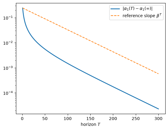
The gap shrinks geometrically, at a rate governed by the spectral radius of \(Q\), which equals \(\beta\).