
130. Affine Models of Asset Prices#
130.1. Overview#
This lecture describes a class of affine or exponential quadratic models of the stochastic discount factor that have become widely used in empirical finance.
These models are presented in chapter 15 of Ljungqvist and Sargent [2018].
The models discussed here take a different approach from the time-separable CRRA stochastic discount factor of Hansen and Singleton [1983], studied in our companion lecture.
The CRRA stochastic discount factor is
where \(\rho\) is the rate of time preference, \(\gamma\) is the coefficient of relative risk aversion, log consumption growth is \(g + \sigma_c \varepsilon_{t+1}\), and \(r_t = \rho + \gamma g - \frac{1}{2}\sigma_c^2\gamma^2\).
This model asserts that exposure to the random part of aggregate consumption growth, \(\sigma_c\varepsilon_{t+1}\), is the only priced risk, the sole source of discrepancies among expected returns across assets.
Empirical difficulties with this specification (the equity premium puzzle, the risk-free rate puzzle, and the Hansen-Jagannathan bounds discussed in Doubts or Variability?) motivate the alternative approach described in this lecture.
Put bluntly, the model to be studied in this lecture declares the Lucas asset pricing model’s stochastic discount factor to be a failure.
The affine model maintains \(\mathbb{E}(m_{t+1}R_{j,t+1}) = 1\) but divorces the stochastic discount factor from consumption risk, and consequently, from much of macroeconomics too.
Instead, it
specifies an analytically tractable stochastic process for \(m_{t+1}\), and
uses overidentifying restrictions from \(\mathbb{E}(m_{t+1}R_{j,t+1}) = 1\) applied to \(N\) assets to let the data reveal risks and their prices.
Note
Researchers including [Bansal and Yaron, 2004] and [Hansen et al., 2008] have been less willing to give up on consumption-based models of the stochastic discount factor.
Key applications we study include:
Pricing risky assets: how risk prices and exposures determine excess returns.
Affine term structure models: bond yields as affine functions of a state vector (Ang and Piazzesi [2003]).
Risk-neutral probabilities: a change-of-measure representation of the pricing equation.
Distorted beliefs: reinterpreting risk price estimates when agents hold systematically biased forecasts (Piazzesi et al. [2015]); see also Risk Aversion or Mistaken Beliefs?.
The lecture uses lognormal pricing tools that also appear in Asset Pricing: Finite State Models and Stochastic Consumption, Risk Aversion, and the Temporal Behavior of Asset Returns.
The change-of-measure arguments rely on likelihood ratios of the kind studied in Likelihood Ratio Processes and Statistical Divergence Measures.
We start with the following imports:
import numpy as np
import matplotlib.pyplot as plt
from collections import namedtuple
from numpy.linalg import eigvals
from scipy.linalg import solve_discrete_lyapunov
from scipy.stats import norm
Matplotlib is building the font cache; this may take a moment.
130.2. The model#
130.2.1. State dynamics and short rate#
The model has two components.
Component 1 is a vector autoregression that describes the state of the economy and the evolution of the short rate:
Here
\(\phi\) is a stable \(m \times m\) matrix,
\(C\) is an \(m \times m\) matrix,
\(\varepsilon_{t+1} \sim \mathcal{N}(0, I)\) is an i.i.d. \(m \times 1\) random vector,
\(z_t\) is an \(m \times 1\) state vector.
Equation (130.2) says that the short rate \(r_t\), the net yield on a one-period risk-free claim, is an affine function of the state \(z_t\).
Component 2 is a vector of risk prices \(\lambda_t\) and an associated stochastic discount factor \(m_{t+1}\):
Here \(\lambda_0\) is \(m \times 1\) and \(\lambda_z\) is \(m \times m\).
The entries of \(\lambda_t\) that multiply corresponding entries of the risks \(\varepsilon_{t+1}\) are called risk prices because they determine how exposures to each risk component affect expected returns (as we show below).
Because \(\lambda_t\) is affine in \(z_t\), the stochastic discount factor \(m_{t+1}\) is exponential quadratic in the state \(z_t\).
We implement the model components as follows.
AffineModel = namedtuple('AffineModel',
    ('μ', 'φ', 'C', 'δ_0', 'δ_1', 'λ_0', 'λ_z', 'm', 'φ_rn', 'μ_rn'))

def create_affine_model(μ, φ, C, δ_0, δ_1, λ_0, λ_z):
    """Create an affine term structure model."""
    μ = np.asarray(μ, float)
    φ = np.asarray(φ, float)
    C = np.asarray(C, float)
    δ_1 = np.asarray(δ_1, float)
    λ_0, λ_z = np.asarray(λ_0, float), np.asarray(λ_z, float)
    return AffineModel(μ=μ, φ=φ, C=C, δ_0=float(δ_0), δ_1=δ_1,
                       λ_0=λ_0, λ_z=λ_z, m=len(μ),
                       φ_rn=φ - C @ λ_z, μ_rn=μ - C @ λ_0)

def simulate(model, z0, T, rng=None):
    """Simulate z_{t+1} = μ + φ z_t + C ε_{t+1} for T periods."""
    if rng is None:
        rng = np.random.default_rng(42)
    Z = np.zeros((T + 1, model.m))
    Z[0] = z0
    for t in range(T):
        ε = rng.standard_normal(model.m)
        Z[t + 1] = model.μ + model.φ @ Z[t] + model.C @ ε
    return Z

def short_rate(model, z):
    """Compute r_t = δ_0 + δ_1^⊤ z_t."""
    return model.δ_0 + model.δ_1 @ z

def risk_prices(model, z):
    """Compute λ_t = λ_0 + λ_z z_t."""
    return model.λ_0 + model.λ_z @ z
130.2.2. Properties of the SDF#
Since \(\lambda_t^\top\varepsilon_{t+1}\) is conditionally normal, it follows that
and
Exercise 130.1
Show that the SDF defined in (130.4) satisfies
and
where \(\| \lambda_t \| = \sqrt{\lambda_t^\top\lambda_t}\) denotes the Euclidean norm of the risk price vector.
For the second result, use the lognormal variance formula and the approximations \(\exp(x) \approx 1 + x\) and \(\exp(-r_t) \approx 1\) for small \(x\) and \(r_t\).
Solution
From (130.4), we have
Since \(-\lambda_t^\top \varepsilon_{t+1} \sim \mathcal{N}(0, \lambda_t^\top \lambda_t)\), we have \(\mathbb{E}_t[\exp(-\lambda_t^\top \varepsilon_{t+1})] = \exp\left(\frac{1}{2}\lambda_t^\top \lambda_t\right)\).
Therefore,
\(m_{t+1}\) is conditionally lognormal with \(\log m_{t+1} \sim \mathcal{N}(-r_t-\frac{1}{2}\lambda_t^\top\lambda_t, \lambda_t^\top \lambda_t)\).
By the lognormal variance formula \(\text{Var}(\exp(X)) = (\exp(\sigma^2) - 1) \exp(2\mu + \sigma^2)\) for \(X \sim \mathcal{N}(\mu, \sigma^2)\), we have
by the approximation \(\exp(x) \approx 1 + x\) for small \(x\).
Hence,
With \(\exp(-r_t) \approx 1\) for small \(r_t\), we obtain
The first equation confirms that \(r_t\) is the net yield on a risk-free one-period bond.
That is why \(r_t\) is called the short rate in the exponential quadratic literature.
The second equation says that the conditional standard deviation of the SDF is approximately the magnitude of the vector of risk prices, a measure of overall market price of risk.
The approximation comes from an exact formula: because \(m_{t+1}\) is conditionally lognormal,
By the Hansen–Jagannathan bound [Hansen and Jagannathan, 1991], this ratio bounds the conditional Sharpe ratio of every excess return, so \(\|\lambda_t\|\) tells us how large Sharpe ratios can be.
130.3. Pricing risky assets#
130.3.1. Lognormal returns#
Consider a risky asset \(j\) whose gross return has a lognormal conditional distribution:
where the exposure vector
Here \(\alpha_0(j)\) is \(m \times 1\) and \(\alpha_z(j)\) is \(m \times m\).
The components of \(\alpha_t(j)\) express the exposures of \(\log R_{j,t+1}\) to corresponding components of the risk vector \(\varepsilon_{t+1}\).
The specification (130.5) implies \(\mathbb{E}_t R_{j,t+1} = \exp(\nu_t(j))\), so \(\nu_t(j)\) is the log of the expected gross return.
130.3.2. Expected excess returns#
Applying the pricing equation \(\mathbb{E}_t(m_{t+1}R_{j,t+1}) = 1\) together with the formula for the mean of a lognormal random variable gives
Exercise 130.2
Using the SDF (130.4) and the return specification (130.5), derive the expected excess return formula (130.7):
Hint: Start by computing \(\log(m_{t+1} R_{j,t+1})\), identify its conditional distribution, and apply the pricing condition \(\mathbb{E}_t(m_{t+1}R_{j,t+1}) = 1\).
Solution
Combining (130.4) and (130.5), we get
This is conditionally normal with mean \(\mu = -r_t + \nu_t(j) - \frac{1}{2}\lambda_t^\top\lambda_t - \frac{1}{2}\alpha_t(j)^\top\alpha_t(j)\) and variance \(\sigma^2 = (\alpha_t(j) - \lambda_t)^\top(\alpha_t(j) - \lambda_t)\).
Since \(\mathbb{E}_t[\exp(X)] = \exp(\mu + \frac{1}{2}\sigma^2)\) for \(X \sim \mathcal{N}(\mu, \sigma^2)\), the pricing condition \(\mathbb{E}_t(m_{t+1}R_{j,t+1}) = 1\) requires \(\mu + \frac{1}{2}\sigma^2 = 0\).
Expanding \(\frac{1}{2}\sigma^2 = \frac{1}{2}\alpha_t(j)^\top\alpha_t(j) - \alpha_t(j)^\top\lambda_t + \frac{1}{2}\lambda_t^\top\lambda_t\) and adding to \(\mu\), the \(\frac{1}{2}\lambda_t^\top\lambda_t\) and \(\frac{1}{2}\alpha_t(j)^\top\alpha_t(j)\) terms cancel, leaving
which gives (130.7).
This is a central result.
It says:
The log expected gross return on asset \(j\) equals the short rate plus the inner product of the asset’s exposure vector \(\alpha_t(j)\) with the risk price vector \(\lambda_t\).
Each component of \(\lambda_t\) prices the corresponding component of \(\varepsilon_{t+1}\).
An asset that loads heavily on a risk component with a large risk price earns a correspondingly high expected return.
Exercise 130.3
Suppose that a representative agent has CRRA utility with risk aversion \(\gamma\) and discount factor \(\beta = e^{-\rho}\), and that log consumption growth is \(\log(c_{t+1}/c_t) = g + \sigma_c^\top \varepsilon_{t+1}\), where \(\sigma_c\) is an \(m \times 1\) vector.
Show that \(m_{t+1} = \beta (c_{t+1}/c_t)^{-\gamma}\) has the form (130.4) with a constant risk price vector \(\lambda_t = \gamma \sigma_c\), and find \(r_t\).
Define the conditional Sharpe ratio of the log return on asset \(j\) as \((\nu_t(j) - r_t)/\|\alpha_t(j)\|\). Use (130.7) and the Cauchy–Schwarz inequality to show that the largest such Sharpe ratio is \(\|\lambda_t\|\), and that it is attained by returns whose exposure vector is proportional to \(\lambda_t\).
Suppose that \(\|\sigma_c\| = 0.02\) per year and that some asset has an annual Sharpe ratio of \(0.4\). Using the exact bound \(\sqrt{\exp(\lambda^\top\lambda) - 1} \geq 0.4\), compute the smallest \(\gamma\) consistent with the CRRA model, and compare it with the first-order answer \(\gamma \geq 0.4 / 0.02\).
Solution
Part 1. Taking logs,
Matching the shock term with (130.4) gives \(\lambda_t = \gamma \sigma_c\).
Matching the constant gives \(-r_t - \frac{1}{2}\gamma^2 \sigma_c^\top\sigma_c = -\rho - \gamma g\), so
This is the CRRA model from the overview, now written as a special case of the affine model with \(\lambda_z = 0\).
Part 2. By (130.7), the Sharpe ratio is \(\alpha_t(j)^\top\lambda_t / \|\alpha_t(j)\|\).
The Cauchy–Schwarz inequality gives \(\alpha_t(j)^\top\lambda_t \leq \|\alpha_t(j)\| \, \|\lambda_t\|\), with equality exactly when \(\alpha_t(j)\) is a positive multiple of \(\lambda_t\).
The following check maximizes the Sharpe ratio over many random exposure vectors.
rng = np.random.default_rng(1234)
λ_example = np.array([0.3, 0.1])
α_draws = rng.standard_normal((20_000, 2))
sharpe = α_draws @ λ_example / np.linalg.norm(α_draws, axis=1)
print(f"largest Sharpe ratio over draws: {sharpe.max():.5f}")
print(f"||λ||:                           {np.linalg.norm(λ_example):.5f}")
largest Sharpe ratio over draws: 0.31623
||λ||:                           0.31623
Part 3.
σ_c_norm, target_sr = 0.02, 0.4
λ_norm_required = np.sqrt(np.log(1 + target_sr**2))
print(f"required ||λ|| (exact bound): {λ_norm_required:.4f}")
print(f"implied γ (exact bound):      {λ_norm_required / σ_c_norm:.1f}")
print(f"implied γ (first order):      {target_sr / σ_c_norm:.1f}")
required ||λ|| (exact bound): 0.3853
implied γ (exact bound):      19.3
implied γ (first order):      20.0
Either way, the CRRA model needs a coefficient of relative risk aversion near \(20\).
This is the equity premium puzzle expressed in the language of this lecture.
The affine model sidesteps the puzzle by treating \(\lambda_t\) as free parameters to be estimated from asset returns rather than tying them to consumption growth.
130.4. Affine term structure of yields#
One of the most important applications is the affine term structure model studied by Ang and Piazzesi [2003].
130.4.1. Bond prices#
Let \(p_t(n)\) be the price at time \(t\) of a risk-free pure discount bond maturing at \(t + n\) (paying one unit of consumption).
The one-period gross return on holding an \((n+1)\)-period bond from \(t\) to \(t+1\) is
The pricing equation \(\mathbb{E}_t(m_{t+1}R_{t+1}) = 1\) implies
with the initial condition
130.4.2. Exponential affine prices#
The recursion (130.8) has an exponential affine solution:
where the scalar \(\bar A_n\) and the \(m \times 1\) vector \(\bar B_n\) satisfy the Riccati difference equations
with initial conditions \(\bar A_1 = -\delta_0\) and \(\bar B_1 = -\delta_1\).
Exercise 130.4
Derive the Riccati difference equations (130.10) and (130.11) by substituting the conjectured bond price (130.9) into the pricing recursion (130.8) and matching coefficients.
Hint: Substitute \(p_{t+1}(n) = \exp(\bar A_n + \bar B_n^\top z_{t+1})\) and \(\log m_{t+1}\) from (130.4) into (130.8).
Use the state dynamics (130.1) to express \(z_{t+1}\) in terms of \(z_t\) and \(\varepsilon_{t+1}\), then evaluate the conditional expectation using the lognormal moment generating function.
Solution
We want to show that if \(p_t(n) = \exp(\bar A_n + \bar B_n^\top z_t)\), then the recursion \(p_t(n+1) = \mathbb{E}_t(m_{t+1}\, p_{t+1}(n))\) yields \(p_t(n+1) = \exp(\bar A_{n+1} + \bar B_{n+1}^\top z_t)\) with \(\bar A_{n+1}\) and \(\bar B_{n+1}\) given by (130.10) and (130.11).
Substituting \(z_{t+1} = \mu + \phi z_t + C\varepsilon_{t+1}\) from (130.1) and \(r_t = \delta_0 + \delta_1^\top z_t\) from (130.2) gives
Since \(\varepsilon_{t+1} \sim \mathcal{N}(0, I)\), and writing the exponent as \(a + b^\top\varepsilon_{t+1}\) where \(b = C^\top \bar B_n - \lambda_t\), we have
Computing \(\frac{1}{2}b^\top b\):
The \(\frac{1}{2}\lambda_t^\top\lambda_t\) cancels with the \(-\frac{1}{2}\lambda_t^\top\lambda_t\) already in \(a\), and \(-\bar B_n^\top C\lambda_t = -\bar B_n^\top C(\lambda_0 + \lambda_z z_t)\).
Matching the constant and the coefficient on \(z_t\) gives the Riccati equations (130.10) and (130.11).
Setting \(n = 0\) with \(p_t(1) = \exp(-r_t) = \exp(-\delta_0 - \delta_1^\top z_t)\) gives \(\bar A_1 = -\delta_0\) and \(\bar B_1 = -\delta_1\).
130.4.3. Yields#
The yield to maturity on an \(n\)-period bond is the constant rate \(y\) at which one would discount the face value to obtain the observed price, i.e., \(p_t(n) = e^{-n\,y}\).
Solving for \(y\) gives
Substituting (130.9) gives
where \(A_n = -\bar A_n / n\) and \(B_n = -\bar B_n / n\).
Yields are affine functions of the state vector \(z_t\).
This is the defining property of affine term structure models.
We now implement the bond pricing formulas (130.10), (130.11), and (130.12).
def bond_coefficients(model, n_max):
    """Compute (A_bar_n, B_bar_n) for n = 1, ..., n_max."""
    A_bar = np.zeros(n_max + 1)
    B_bar = np.zeros((n_max + 1, model.m))
    A_bar[1], B_bar[1] = -model.δ_0, -model.δ_1
    CC = model.C @ model.C.T
    for n in range(1, n_max):
        Bn = B_bar[n]
        A_bar[n + 1] = (A_bar[n] + Bn @ model.μ_rn
                       + 0.5 * Bn @ CC @ Bn
                       - model.δ_0)
        B_bar[n + 1] = model.φ_rn.T @ Bn - model.δ_1
    return A_bar, B_bar

def compute_yields(model, z, n_max):
    """Compute yield curve y_t(n) for n = 1, ..., n_max."""
    A_bar, B_bar = bond_coefficients(model, n_max)
    return np.array([(-A_bar[n] - B_bar[n] @ z) / n
                     for n in range(1, n_max + 1)])

def bond_prices(model, z, n_max):
    """Compute bond prices p_t(n) for n = 1, ..., n_max."""
    A_bar, B_bar = bond_coefficients(model, n_max)
    return np.array([np.exp(A_bar[n] + B_bar[n] @ z)
                     for n in range(1, n_max + 1)])
130.4.4. A one-factor Gaussian example#
To build intuition, we start with a single-factor (\(m=1\)) Gaussian model.
With \(m = 1\), the state \(z_t\) follows an AR(1) process \(z_{t+1} = \mu + \phi z_t + C\varepsilon_{t+1}\).
The unconditional standard deviation of \(z_t\) is \(\sigma_z = C / \sqrt{1 - \phi^2}\), which determines the range of short rates the model generates via \(r_t = \delta_0 + \delta_1 z_t\).
# One-factor Gaussian model (quarterly)
μ      = np.array([0.0])
φ      = np.array([[0.95]])
C      = np.array([[1.0]])
δ_0    = 0.01                  # 1%/quarter ≈ 4% p.a.
δ_1    = np.array([0.001])
λ_0    = np.array([-0.05])
λ_z    = np.array([[-0.01]])

model_1f = create_affine_model(μ, φ, C, δ_0, δ_1, λ_0, λ_z)
130.4.5. Yield curve shapes#
We compute yield curves \(y_t(n)\) across a range of short-rate states \(z_t\).
n_max_1f = 200
maturities_1f = np.arange(1, n_max_1f + 1)

z_low  = np.array([-5.0])
z_mid  = np.array([0.0])
z_high = np.array([5.0])

fig, ax = plt.subplots(figsize=(9, 5.5))

r_low = short_rate(model_1f, z_low) * 4 * 100
r_mid = short_rate(model_1f, z_mid) * 4 * 100
r_high = short_rate(model_1f, z_high) * 4 * 100

for z, label in [
    (z_low,  f"Low state  ($y_t(1) = ${r_low:.1f}%)"),
    (z_mid,  f"Median state ($y_t(1) = ${r_mid:.1f}%)"),
    (z_high, f"High state ($y_t(1) = ${r_high:.1f}%)"),
]:
    y = compute_yields(model_1f, z, n_max_1f) * 4 * 100
    line, = ax.plot(maturities_1f, y, lw=2.2, label=label)
    ax.plot(1, y[0], 'o', color=line.get_color(), ms=7, zorder=5)

r_bar = short_rate(model_1f, np.array([0.0])) * 4 * 100
ax.axhline(r_bar, color='grey', ls=':', lw=1.2, alpha=0.7,
           label=f"Mean short rate ({r_bar:.1f}%)")

# Long-run yield: B_bar_n converges, so y_inf = lim -A_bar_n / n
φ_Cλ = (model_1f.φ_rn)[0, 0]          # φ - Cλ_z (scalar)
B_inf = -model_1f.δ_1[0] / (1 - φ_Cλ) # fixed point of B recursion
A_increment = (B_inf * model_1f.μ_rn[0]
               + 0.5 * B_inf**2 * (model_1f.C @ model_1f.C.T)[0, 0]
               - model_1f.δ_0)
y_inf = -A_increment * 4 * 100         # annualised %
ax.axhline(y_inf, color='black', ls='--', lw=1.2, alpha=0.7,
           label=f"Long-run yield ({y_inf:.1f}%)")

ax.set_xlabel("Maturity (quarters)")
ax.set_ylabel("Yield (% per annum)")
ax.legend(fontsize=10, loc='best')
ax.set_xlim(1, n_max_1f)

ax2 = ax.twiny()
ax2.set_xlim(ax.get_xlim())
year_ticks = [4, 40, 80, 120, 160, 200]
ax2.set_xticks(year_ticks)
ax2.set_xticklabels([f"{t/4:.0f}y" for t in year_ticks])
ax2.set_xlabel("Maturity (years)")

plt.tight_layout()
plt.show()
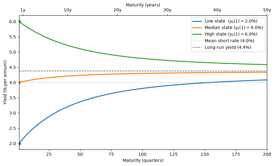
Fig. 130.1 Yield curves under the one-factor affine model#
When the short rate is low, the yield curve is upward-sloping, while when the short rate is high, it is downward-sloping.
All three curves approach the same long-run yield \(y_\infty\), which lies above the mean short rate \(\delta_0\).
The approach is slow.
Because \(\bar B_n\) converges to a finite limit, the state enters \(y_t(n)\) through \(\bar B_n^\top z_t / n\), so gaps between curves shrink only at rate \(1/n\).
That is why we plot maturities out to 50 years: at 15 years the three curves are still spread between about 3.5% and 5.0%, while at 50 years they lie between about 4.1% and 4.6%.
Exercise 130.5
Show that the long-run yield satisfies
where \(\bar B_\infty = -(I - (\phi - C\lambda_z)^\top)^{-1} \delta_1\) is the fixed point of the recursion (130.11).
Then explain why \(y_\infty > \delta_0\) under this parameterization.
Hint: Use (130.12) and the Riccati equations (130.10)–(130.11).
For the inequality, consider each subtracted term separately.
Solution
The recursion (130.11) is a linear difference equation \(\bar B_{n+1} = (\phi - C\lambda_z)^\top \bar B_n - \delta_1\).
When \(\phi - C\lambda_z\) has eigenvalues inside the unit circle, \(\bar B_n\) converges to \(\bar B_\infty = -(I - (\phi - C\lambda_z)^\top)^{-1} \delta_1\).
Since \(\bar B_\infty\) is finite, \(\bar B_n^\top z_t / n \to 0\) in (130.12), so \(y_t(n) \to \lim_{n\to\infty} -\bar A_n / n\) regardless of \(z_t\).
To find this limit, write \(\bar A_n = \bar A_1 + \sum_{k=1}^{n-1}(\bar A_{k+1} - \bar A_k)\).
By (130.10), each increment depends on \(\bar B_k\), which converges to \(\bar B_\infty\), so the increment converges to \(L \equiv \bar B_\infty^\top(\mu - C\lambda_0) + \tfrac{1}{2}\bar B_\infty^\top CC^\top \bar B_\infty - \delta_0\).
Therefore \(\bar A_n / n \to L\) and \(y_\infty = -L\), giving (130.13).
To see why \(y_\infty > \delta_0\), note that the two subtracted terms in (130.13) have opposite signs under this parameterization.
The quadratic term \(\tfrac{1}{2}\bar B_\infty^\top CC^\top \bar B_\infty = \tfrac{1}{2}\|C^\top \bar B_\infty\|^2 \geq 0\) always.
This is a convexity effect from Jensen’s inequality that pushes \(y_\infty\) below \(\delta_0\).
The linear term \(\bar B_\infty^\top(\mu - C\lambda_0)\) is negative because \(\bar B_\infty < 0\) (since \(\delta_1 > 0\)) while \(\mu - C\lambda_0 > 0\) (since \(\lambda_0 < 0\)).
Subtracting this negative quantity raises \(y_\infty\) above \(\delta_0\).
This is a risk-premium effect: positive term premiums tilt the average yield curve upward.
Under this parameterization the risk-premium effect dominates the convexity effect, so \(y_\infty > \delta_0\).
Let’s also simulate the short rate path:
T = 200
Z = simulate(model_1f, np.array([0.0]), T)
short_rates = np.array([short_rate(model_1f, Z[t]) * 4 * 100
                        for t in range(T + 1)])
r_bar_pct = short_rate(model_1f, np.array([0.0])) * 4 * 100

fig, ax = plt.subplots(figsize=(10, 4))
quarters = np.arange(T + 1)
line, = ax.plot(quarters, short_rates, lw=1.3)
ax.axhline(r_bar_pct, ls="--", lw=1.3,
           label=f"Unconditional mean ({r_bar_pct:.1f}%)")
ax.fill_between(quarters, short_rates, r_bar_pct,
                alpha=0.08, color=line.get_color())
ax.set_xlabel("Quarter")
ax.set_ylabel("Short rate (% p.a.)")
ax.set_xlim(0, T)
ax.legend(fontsize=11)
plt.tight_layout()
plt.show()
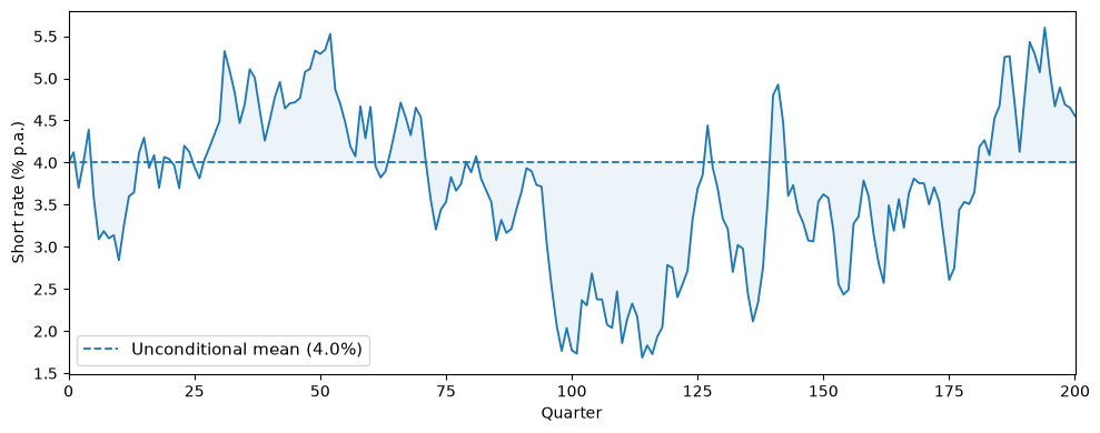
Fig. 130.2 Simulated short rate path#
Because \(r_t\) is an affine function of a Gaussian state, a Gaussian affine model assigns positive probability to negative short rates.
Under the stationary distribution of the one-factor model, \(r_t\) is normal with mean \(\delta_0\) and standard deviation \(\delta_1 \sigma_z\), which lets us compute that probability.
σ_z = model_1f.C[0, 0] / np.sqrt(1 - model_1f.φ[0, 0]**2)
σ_r = model_1f.δ_1[0] * σ_z
print(f"Stationary std of r_t: {σ_r * 4 * 100:.2f}% p.a.")
print(f"P(r_t < 0):            {norm.cdf(-model_1f.δ_0 / σ_r):.2e}")
Stationary std of r_t: 1.28% p.a.
P(r_t < 0):            8.97e-04
The probability is small in this calibration, but it can be substantial in calibrations fit to periods of low interest rates.
Square-root models such as Cox et al. [1985] and shadow-rate models such as Black [1995] are two ways of keeping nominal rates non-negative, at the cost of some of the tractability that the Gaussian specification delivers.
130.4.6. A two-factor model#
To match richer yield-curve dynamics, practitioners routinely use \(m \geq 2\) factors.
We now introduce a two-factor specification with state \(z_t = (z_{1t},\, z_{2t})^\top\), where
The first factor \(z_{1t}\) is highly persistent (\(\phi_{11} = 0.97\)) and drives most of the variation in the short rate through \(\delta_1\), so we interpret it as a level factor.
The second factor \(z_{2t}\) mean-reverts faster (\(\phi_{22} = 0.90\)) and affects the short rate with a smaller loading, capturing the slope of the yield curve.
The off-diagonal entry \(\phi_{12} = -0.03\) allows the level factor to respond to the current slope state \(z_{2t}\).
The short rate is \(r_t = \delta_0 + \delta_1^\top z_t\) with \(\delta_1 = (0.002,\; 0.001)^\top\), so both factors raise the short rate when positive, but the level factor has twice the impact.
Risk prices are \(\lambda_t = \lambda_0 + \lambda_z z_t\) with \(\lambda_0 = (-0.01,\; -0.005)^\top\) and \(\lambda_z = \text{diag}(-0.005,\, -0.003)\).
The negative diagonal entries of \(\lambda_z\) make \(\phi - C\lambda_z\) have larger eigenvalues than \(\phi\), so the state is more persistent under the risk-neutral measure and the yield curve is more sensitive to the current state at long horizons.
# Two-factor model: z = [level, slope]
μ_2  = np.array([0.0,  0.0])
φ_2  = np.array([[0.97, -0.03],
                  [0.00,  0.90]])
C_2  = np.eye(2)
δ_0_2 = 0.01
δ_1_2 = np.array([0.002, 0.001])
λ_0_2 = np.array([-0.01, -0.005])
λ_z_2 = np.array([[-0.005, 0.0],
                   [ 0.0, -0.003]])

model_2f = create_affine_model(μ_2, φ_2, C_2, δ_0_2, δ_1_2, λ_0_2, λ_z_2)

print(f"Eigenvalues of φ:       {eigvals(φ_2).real.round(4)}")
print(f"Eigenvalues of φ - Cλ_z: {eigvals(model_2f.φ_rn).real.round(4)}")
Eigenvalues of φ:       [0.97 0.9 ]
Eigenvalues of φ - Cλ_z: [0.975 0.903]
This confirms that the eigenvalues of \(\phi - C\lambda_z\) are larger than those of \(\phi\), so the state is more persistent under the risk-neutral measure.
The following figure shows yield curves across different states of the world, as well as the factor loadings \(B_{n,1}\) and \(B_{n,2}\) that determine how yields load on the level and slope factors at each maturity
n_max_2f = 60
maturities_2f = np.arange(1, n_max_2f + 1)

states = {
    "Normal":              np.array([0.0,   0.0]),
    "Low short rate":      np.array([-4.0,  3.0]),
    "High short rate":     np.array([4.0,  -3.0]),
}

fig, (ax1, ax2) = plt.subplots(1, 2, figsize=(14, 5.5))

for label, z in states.items():
    r_now = short_rate(model_2f, z) * 4 * 100
    y = compute_yields(model_2f, z, n_max_2f) * 4 * 100
    line, = ax1.plot(maturities_2f, y, lw=2.2,
                     label=f"{label} (r₁ = {r_now:.1f}%)")
    ax1.plot(1, y[0], 'o', color=line.get_color(), ms=7, zorder=5)

ax1.set_xlabel("Maturity (quarters)")
ax1.set_ylabel("Yield (% p.a.)")
ax1.legend(fontsize=10)
ax1.set_xlim(1, n_max_2f)

A_bar, B_bar = bond_coefficients(model_2f, n_max_2f)
ns = np.arange(1, n_max_2f + 1)
B_n = np.array([-B_bar[n] / n for n in ns])

ax2.plot(ns, B_n[:, 0], lw=2.2,
         label=r"Level loading $B_{n,1}$")
ax2.plot(ns, B_n[:, 1], lw=2.2,
         label=r"Slope loading $B_{n,2}$")
ax2.axhline(0, color='black', lw=0.6)
ax2.set_xlabel("Maturity (quarters)")
ax2.set_ylabel(r"Yield loading $B_{n,k}$")
ax2.legend(fontsize=11)
ax2.set_xlim(1, n_max_2f)

for ax in (ax1, ax2):
    ax_top = ax.twiny()
    ax_top.set_xlim(ax.get_xlim())
    year_ticks = [4, 12, 20, 40, 60]
    ax_top.set_xticks(year_ticks)
    ax_top.set_xticklabels([f"{t/4:.0f}y" for t in year_ticks])

plt.tight_layout()
plt.show()
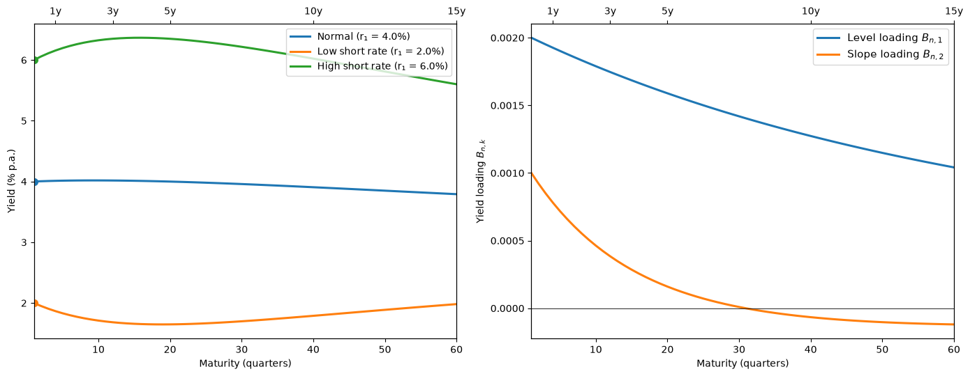
Fig. 130.3 Yield curves and factor loadings under the two-factor model#
The right panel shows how yields at different maturities respond to the two factors.
The level loading \(B_{n,1}\) declines gradually with maturity, from \(0.002\) at one quarter to about half that at 15 years, so the persistent factor moves yields at all maturities.
The slope loading \(B_{n,2}\) starts at \(0.001\), decays quickly, and turns slightly negative beyond about 30 quarters.
The sign change reflects the off-diagonal entry \(\phi_{12} = -0.03\): a high \(z_{2t}\) raises the short rate today but pushes the level factor, and hence future short rates, down.
As a result, the level factor dominates yields at long maturities, while the slope factor matters mainly at the short end.
As in the one-factor case, the curves in the left panel are still approaching their common long-run yield at 60 quarters.
130.5. Risk premiums#
A key object in the affine term structure model is the term premium, the expected excess return on a long-term bond relative to rolling over short-term bonds.
For an \((n+1)\)-period bond held for one period, the shock loading is \(\alpha_n = C^\top \bar B_n\), so (130.7) gives
The term premium equals the inner product of the bond’s shock exposure \(\bar B_n^\top C\) with the risk price vector \(\lambda_t\).
This formula measures the premium as the log of an expected gross return.
The expected log excess return is smaller by a Jensen’s inequality term:
Only the first term depends on the state, so the two measures differ by a maturity-specific constant that does not affect how term premiums vary over time.
Because the term premium equals \(\bar B_n^\top C \lambda_t\), its sign depends on the current risk-price vector \(\lambda_t\), which is state-dependent whenever \(\lambda_z \neq 0\).
To see this more concretely, consider a state where \(C\lambda_t\) is negative componentwise (for example, \(z_t = 0\) in our calibration below).
When \(\delta_1 > 0\), a positive shock \(\varepsilon_{t+1}\) raises the short rate and lowers long-bond prices, so the bond shock loading \(\alpha_n = C^\top \bar B_n\) is negative.
A negative \(C\lambda_t\) then means the stochastic discount factor \(m_{t+1}\) loads positively on \(\varepsilon_{t+1}\), i.e. the SDF is high in states where interest rates rise and bond prices fall.
This makes \(\text{Cov}_t(m_{t+1}, R_{t+1}^{(n+1)}) < 0\), so long bonds are risky and carry a positive term premium.
Algebraically, \(\bar B_n < 0\) and \(C\lambda_t < 0\) combine to give \(\bar B_n^\top C \lambda_t > 0\).
In other states, however, components of \(\lambda_t\) can change sign.
With \(\lambda_z < 0\), a low value of the level factor \(z_{1t}\) pushes the first component of \(\lambda_t\) above zero.
Since long bonds load mainly on the level shock, their term premiums then turn negative.
Exercise 130.6
Derive the term premium formula above by computing the one-period holding return on an \((n+1)\)-period bond and identifying its shock loading.
Hint: Use \(R_{t+1}^{(n+1)} = p_{t+1}(n)/p_t(n+1)\) with \(\log p_t(n) = \bar A_n + \bar B_n^\top z_t\), substitute the state dynamics (130.1), and apply the Riccati equations (130.10)–(130.11) to simplify.
Solution
The one-period holding return on an \((n+1)\)-period bond is \(R_{t+1}^{(n+1)} = p_{t+1}(n)/p_t(n+1)\), so
Substituting \(z_{t+1} = \mu + \phi z_t + C\varepsilon_{t+1}\) from (130.1):
We now use the Riccati equations to simplify each piece.
For the constant piece, (130.10) gives \(\bar A_{n+1} = \bar A_n + \bar B_n^\top(\mu - C\lambda_0) + \tfrac{1}{2}\bar B_n^\top CC^\top \bar B_n - \delta_0\), so
For the \(z_t\) coefficient, (130.11) gives \(\bar B_{n+1}^\top = \bar B_n^\top(\phi - C\lambda_z) - \delta_1^\top\), so
Combining the pieces:
Writing \(\alpha_n = C^\top \bar B_n\), this takes the generic return form (130.5):
Since \(\mathbb{E}_t R_{t+1}^{(n+1)} = \exp(\nu_t)\), we obtain
The following figure plots term premiums across maturities for different states of the world, as well as the level and slope factor contributions to the term premium in the normal state
def term_premiums(model, z, n_max):
    """
    Compute one-period term premiums on bonds of maturity 1, ..., n_max.

    An n-period bond held for one period becomes an (n-1)-period bond,
    so its premium is B_bar_{n-1}^⊤ C λ_t (and zero for n = 1).
    """
    A_bar, B_bar = bond_coefficients(model, n_max + 1)
    λ_t = risk_prices(model, z)
    return np.array([B_bar[n-1] @ model.C @ λ_t
                     for n in range(1, n_max + 1)])

n_max_tp = 60
maturities_tp = np.arange(1, n_max_tp + 1)

z_states_tp = {
    "Low rate ($z_1 < 0$)":  np.array([-3.0, 2.0]),
    "High rate ($z_1 > 0$)": np.array([3.0, -2.0]),
}

fig, (ax1, ax2) = plt.subplots(1, 2, figsize=(14, 5.5))

for label, z in z_states_tp.items():
    tp = term_premiums(model_2f, z, n_max_tp) * 4 * 100
    r_now = short_rate(model_2f, z) * 4 * 100
    lam = risk_prices(model_2f, z)
    ax1.plot(maturities_tp, tp, lw=2.2,
             label=(f"{label}\n  r={r_now:.1f}%,"
                    f" λ=[{lam[0]:.3f}, {lam[1]:.3f}]"))

ax1.axhline(0, color="black", lw=0.8, ls="--")
ax1.set_xlabel("Maturity (quarters)")
ax1.set_ylabel("Term premium (% p.a.)")
ax1.legend(fontsize=9)
ax1.set_xlim(1, n_max_tp)

z_decomp = np.array([0.0, 0.0])
A_bar_d, B_bar_d = bond_coefficients(model_2f, n_max_tp + 1)
λ_t = risk_prices(model_2f, z_decomp)
C_lam = model_2f.C @ λ_t

tp_level = np.array([B_bar_d[n-1, 0] * C_lam[0]
                      for n in range(1, n_max_tp + 1)]) * 4 * 100
tp_slope = np.array([B_bar_d[n-1, 1] * C_lam[1]
                      for n in range(1, n_max_tp + 1)]) * 4 * 100
tp_total = tp_level + tp_slope

ax2.plot(maturities_tp, tp_total, 'k-', lw=2.2, label="Total")
ax2.plot(maturities_tp, tp_level, lw=1.8, ls="--",
         label="Level factor")
ax2.plot(maturities_tp, tp_slope, lw=1.8, ls="--",
         label="Slope factor")
ax2.axhline(0, color="black", lw=0.6, ls=":")
ax2.set_xlabel("Maturity (quarters)")
ax2.set_ylabel("Term premium (% p.a.)")
ax2.legend(fontsize=10)
ax2.set_xlim(1, n_max_tp)

for ax in (ax1, ax2):
    ax_top = ax.twiny()
    ax_top.set_xlim(ax.get_xlim())
    year_ticks = [4, 12, 20, 40, 60]
    ax_top.set_xticks(year_ticks)
    ax_top.set_xticklabels([f"{t/4:.0f}y" for t in year_ticks])

plt.tight_layout()
plt.show()
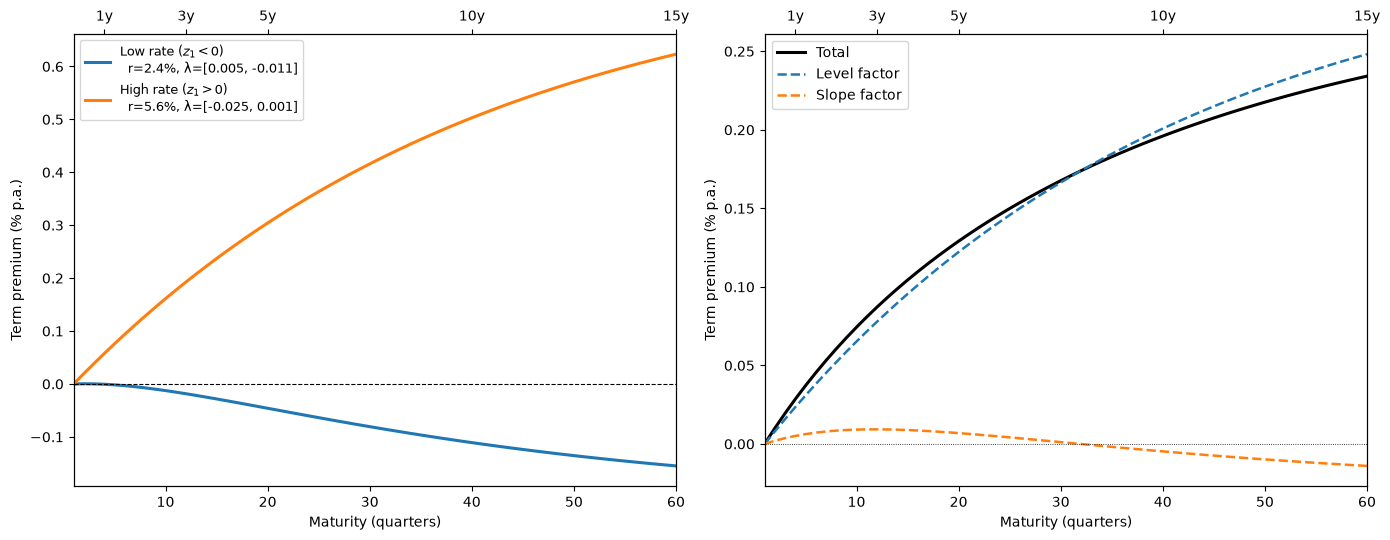
Fig. 130.4 Term premiums and factor decomposition under the two-factor model#
The left panel shows that the sign of the term premium depends on the state.
In the high-rate state, \(\lambda_t \approx (-0.025, 0.001)\), and the term premium is positive and rises with maturity, reaching about 0.6% per year at 15 years.
In the low-rate state, the first component of \(\lambda_t\) has turned positive, \(\lambda_t \approx (0.005, -0.011)\), and the term premium is negative at every maturity, falling to about \(-0.15\)% per year at 15 years.
Investors in the low-rate state accept a lower expected return on long bonds than on rolling over short bonds because long bonds pay off well in the states that they value most.
The right panel decomposes the term premium at \(z_t = 0\), where both components of \(\lambda_t\) are negative.
The level factor accounts for almost all of the premium at long maturities.
The slope contribution is small and turns negative beyond about 30 quarters, mirroring the sign change in the slope loading shown earlier.
Exercise 130.7
The expectations hypothesis says that expected excess returns on long bonds are constant over time, so that they cannot be forecast by the yield spread.
Simulate the two-factor model
model_2ffor \(T = 200{,}000\) quarters. Regress the one-quarter excess holding return on a 20-quarter bond, \(\log p_{t+1}(19) - \log p_t(20) - r_t\), on a constant and the spread \(y_t(20) - r_t\).Compute the population regression slope implied by the model, using \(\bar B_n\) and the stationary covariance matrix \(\Sigma_z\) of \(z_t\), and compare it with your estimate.
Repeat both steps with \(\lambda_z = 0\) and explain the result.
In U.S. data, Fama and Bliss [1987] and Campbell and Shiller [1991] find that high spreads forecast high excess returns on long bonds. Does
model_2freproduce this pattern? What happens if you flip the sign of \(\lambda_z\)?
Solution
From (130.7) and the term-premium formula, the log excess holding return on a 20-quarter bond is
Its conditional mean is a constant plus \(a^\top z_t\) with \(a = \lambda_z^\top C^\top \bar B_{19}\).
The spread is \(s_t = y_t(20) - r_t = \text{constant} + b^\top z_t\) with \(b = -\bar B_{20}/20 - \delta_1\).
Because \(\varepsilon_{t+1}\) is orthogonal to \(z_t\), the population slope is
where \(\Sigma_z\) solves \(\Sigma_z = \phi \Sigma_z \phi^\top + CC^\top\).
def eh_regression(model, n=20, T=200_000, seed=1):
    """OLS and population slopes of excess returns on the yield spread."""
    A_bar, B_bar = bond_coefficients(model, n)
    z_bar = np.linalg.solve(np.eye(model.m) - model.φ, model.μ)
    Z = simulate(model, z_bar, T, rng=np.random.default_rng(seed))

    r = model.δ_0 + Z[:-1] @ model.δ_1
    log_p = lambda k, z: A_bar[k] + z @ B_bar[k]
    excess = log_p(n - 1, Z[1:]) - log_p(n, Z[:-1]) - r
    spread = -log_p(n, Z[:-1]) / n - r

    X = np.column_stack([np.ones(T), spread])
    coef = np.linalg.lstsq(X, excess, rcond=None)[0]
    resid = excess - X @ coef
    se = np.sqrt(resid.var() / (T * spread.var()))

    Σ_z = solve_discrete_lyapunov(model.φ, model.C @ model.C.T)
    a = model.λ_z.T @ model.C.T @ B_bar[n - 1]
    b = -B_bar[n] / n - model.δ_1
    β_pop = (a @ Σ_z @ b) / (b @ Σ_z @ b)
    return coef[1], se, β_pop

cases = {
    "λ_z as calibrated": λ_z_2,
    "λ_z = 0":           np.zeros((2, 2)),
    "λ_z sign flipped":  -λ_z_2,
}
print(f"{'case':>20}  {'OLS slope':>10}  {'s.e.':>7}  {'population':>10}")
for label, lz in cases.items():
    mod = create_affine_model(μ_2, φ_2, C_2, δ_0_2, δ_1_2, λ_0_2, lz)
    b_ols, se, b_pop = eh_regression(mod)
    print(f"{label:>20}  {b_ols:>10.4f}  {se:>7.4f}  {b_pop:>10.4f}")
                case   OLS slope     s.e.  population
   λ_z as calibrated     -0.1614   0.0280     -0.1723
             λ_z = 0      0.0112   0.0250      0.0000
    λ_z sign flipped      0.1728   0.0224      0.1618
With the calibrated \(\lambda_z\), the OLS slope is close to the population slope of about \(-0.17\) and is many standard errors from zero, so the expectations hypothesis fails in simulated data.
With \(\lambda_z = 0\), the vector \(a\) is zero, so expected excess returns are constant and the population slope is exactly zero.
The OLS estimate is then within sampling error of zero.
The expectations hypothesis holds in an affine model exactly when risk prices do not vary with the state.
The calibrated model gets the sign of the Fama–Bliss and Campbell–Shiller finding wrong: a high spread forecasts a low excess return.
Flipping the sign of \(\lambda_z\) reverses the sign of the slope, which shows that the regression evidence is informative about \(\lambda_z\) and not just about the size of average term premiums.
130.6. Risk-neutral probabilities#
We return to the VAR and short-rate equations (130.1)–(130.2), which for convenience we repeat here:
where \(\varepsilon_{t+1} \sim \mathcal{N}(0, I)\).
We suppose that this structure describes the data-generating mechanism.
Finance economists call this the physical measure \(P\), to distinguish it from the risk-neutral measure \(Q\) that we now describe.
Under the physical measure, the conditional distribution of \(z_{t+1}\) given \(z_t\) is \(\mathcal{N}(\mu + \phi z_t,\; CC^\top)\).
130.6.1. Change of measure#
With the risk-price vector \(\lambda_t = \lambda_0 + \lambda_z z_t\) from (130.3), define the non-negative random variable
This is a log-normal random variable with mean 1, so it is a valid likelihood ratio that can be used to twist the conditional distribution of \(z_{t+1}\).
To see what the twist does to the shocks, multiply the standard normal density of \(\varepsilon_{t+1}\) by (130.14):
So under \(Q\) the shock is \(\varepsilon_{t+1} \sim \mathcal{N}(-\lambda_t, I)\): the twist shifts its mean by \(-\lambda_t\) and leaves its covariance matrix unchanged.
Substituting \(\varepsilon_{t+1} = -\lambda_t + \varepsilon^Q_{t+1}\) into (130.1) shows that multiplying the physical conditional distribution by this likelihood ratio transforms it into the risk-neutral conditional distribution
In other words, under \(Q\) the state follows
where \(\varepsilon^Q_{t+1} \sim \mathcal{N}(0, I)\) under \(Q\).
The risk-neutral distribution twists the conditional mean from \(\mu + \phi z_t\) to \(\mu - C\lambda_0 + (\phi - C\lambda_z)z_t\).
The adjustments \(-C\lambda_0\) (constant) and \(-C\lambda_z\) (state-dependent) encode how the pricing equation \(\mathbb{E}^P_t m_{t+1} R_{j,t+1} = 1\) adjusts expected returns for exposure to the risks \(\varepsilon_{t+1}\).
Exercise 130.8
How different are the risk-neutral and physical measures?
A natural measure is relative entropy (Kullback–Leibler divergence), discussed in Statistical Divergence Measures.
Show that the conditional relative entropy of \(Q\) with respect to \(P\), \(\mathbb{E}^Q_t\left[\log(\xi^Q_{t+1}/\xi^Q_t)\right]\), and the conditional relative entropy of \(P\) with respect to \(Q\), \(\mathbb{E}^P_t\left[-\log(\xi^Q_{t+1}/\xi^Q_t)\right]\), both equal \(\tfrac{1}{2}\lambda_t^\top\lambda_t\).
Suppose that \(z_0\) is drawn from the stationary distribution of \(z_t\) under \(P\). Show that the relative entropy of \(P\) with respect to \(Q\) for a sample \(z_1, \ldots, z_T\) equals \(T\) times $\( \tfrac{1}{2}\left(\bar\lambda^\top\bar\lambda + \operatorname{tr}(\lambda_z \Sigma_z \lambda_z^\top)\right) \)\( where \)\bar z = (I - \phi)^{-1}\mu\(, \)\bar\lambda = \lambda_0 + \lambda_z \bar z\(, and \)\Sigma_z\( solves \)\Sigma_z = \phi\Sigma_z\phi^\top + CC^\top$.
Evaluate this formula for
model_2f, verify it by simulation, and use Pinsker’s inequality to bound how well any test based on 100 years of quarterly data on \(z_t\) could distinguish \(P\) from \(Q\).
Solution
Part 1. We showed above that \(\varepsilon_{t+1} \sim \mathcal{N}(-\lambda_t, I)\) under \(Q\), while \(\varepsilon_{t+1} \sim \mathcal{N}(0, I)\) under \(P\).
Hence
and
The two divergences coincide because the two conditional distributions are normal with the same covariance matrix.
Part 2. When \(C\) is invertible, the path \(z_1, \ldots, z_T\) and the shocks \(\varepsilon_1, \ldots, \varepsilon_T\) determine each other given \(z_0\).
The log likelihood ratio of the path is therefore the sum of the one-period log likelihood ratios, and by the law of iterated expectations its expectation under \(P\) is \(\sum_{t=0}^{T-1} \mathbb{E}^P\left[\tfrac{1}{2}\lambda_t^\top\lambda_t\right]\).
Under the stationary distribution, \(\lambda_t = \bar\lambda + \lambda_z(z_t - \bar z)\) with \(\mathbb{E}(z_t - \bar z) = 0\) and \(\text{Var}(z_t) = \Sigma_z\).
Therefore \(\mathbb{E}(\lambda_t^\top\lambda_t) = \bar\lambda^\top\bar\lambda + \operatorname{tr}(\lambda_z\Sigma_z\lambda_z^\top)\) for every \(t\), which gives the formula.
Part 3. Pinsker’s inequality says that the total variation distance between two distributions is at most \(\sqrt{D/2}\), where \(D\) is their relative entropy.
With equal prior probabilities on \(P\) and \(Q\), the smallest achievable probability of choosing the wrong model is \((1 - \text{TV})/2\), so it is at least \((1 - \sqrt{D/2})/2\).
z_bar_2 = np.linalg.solve(np.eye(2) - model_2f.φ, model_2f.μ)
Σ_z_2 = solve_discrete_lyapunov(model_2f.φ, model_2f.C @ model_2f.C.T)
λ_bar_2 = risk_prices(model_2f, z_bar_2)
entropy = 0.5 * (λ_bar_2 @ λ_bar_2
                 + np.trace(model_2f.λ_z @ Σ_z_2 @ model_2f.λ_z.T))

Z_sim = simulate(model_2f, z_bar_2, 200_000, rng=np.random.default_rng(7))
Λ_sim = model_2f.λ_0 + Z_sim @ model_2f.λ_z.T
entropy_sim = 0.5 * np.mean(np.sum(Λ_sim**2, axis=1))

T_years = 100
D = 4 * T_years * entropy
print(f"relative entropy per quarter (formula):    {entropy:.6f}")
print(f"relative entropy per quarter (simulation): {entropy_sim:.6f}")
print(f"relative entropy over {T_years} years:           {D:.4f}")
print(f"lower bound on error probability:          {(1 - np.sqrt(D / 2)) / 2:.3f}")
relative entropy per quarter (formula):    0.000312
relative entropy per quarter (simulation): 0.000310
relative entropy over 100 years:           0.1250
lower bound on error probability:          0.375
Even with a century of quarterly data, no test can push the average probability of choosing the wrong model below about 37%.
Yet the gap between these two hard-to-distinguish measures is exactly what generates the term premiums plotted above.
Time-series data on the state alone therefore say little about risk prices, which is why estimates of \(\lambda_0\) and \(\lambda_z\) rely heavily on the cross-section of bond yields.
This echoes the detection-error calculations of Doubts or Variability?, where plausible amounts of model uncertainty are calibrated in the same way.
130.6.2. Asset pricing in a nutshell#
Let \(\mathbb{E}^P\) denote an expectation under the physical measure that nature uses to generate the data.
Our key asset pricing equation is \(\mathbb{E}^P_t m_{t+1} R_{j,t+1} = 1\) for all returns \(R_{j,t+1}\).
Using (130.14), we can express the SDF (130.4) as
Then the condition \(\mathbb{E}^P_t\bigl(\exp(-r_t)\, \tfrac{\xi^Q_{t+1}}{\xi^Q_t}\, R_{j,t+1}\bigr) = 1\) is equivalent to
Under the risk-neutral measure, expected returns on all assets equal the risk-free return.
130.6.3. Verification via risk-neutral pricing#
Bond prices can be computed by discounting at \(r_t\) under \(Q\):
We can verify that this agrees with (130.9) by iterating the affine recursion under the risk-neutral VAR.
Below we confirm this numerically
def bond_price_mc_Q(model, z0, n, n_sims=50_000, rng=None):
    """Estimate p_t(n) by Monte Carlo under Q; return estimate and std. error."""
    if rng is None:
        rng = np.random.default_rng(0)
    m = len(z0)
    Z = np.tile(z0, (n_sims, 1))
    disc = np.zeros(n_sims)
    for _ in range(n):
        disc += model.δ_0 + Z @ model.δ_1
        ε = rng.standard_normal((n_sims, m))
        Z = model.μ_rn + Z @ model.φ_rn.T + ε @ model.C.T
    payoffs = np.exp(-disc)
    return payoffs.mean(), payoffs.std() / np.sqrt(n_sims)

z_test = np.array([0.01, 0.005])
p_analytic = bond_prices(model_2f, z_test, 40)

rng = np.random.default_rng(0)
maturities_check = [4, 12, 24, 40]
mc_results = [bond_price_mc_Q(model_2f, z_test, n, n_sims=100_000, rng=rng)
              for n in maturities_check]

header = (f"{'Maturity':>10}  {'Analytic':>10}  {'Monte Carlo':>11}"
          f"  {'Error (bps)':>11}  {'s.e. (bps)':>10}  {'z-score':>8}")
print(header)
print("-" * len(header))
for n, (mc, se) in zip(maturities_check, mc_results):
    analytic = p_analytic[n - 1]
    error_bp = (mc - analytic) / analytic * 10_000
    se_bp = se / analytic * 10_000
    print(f"{n:>10}  {analytic:>10.6f}  {mc:>11.6f}"
          f"  {error_bp:>11.2f}  {se_bp:>10.2f}  {error_bp / se_bp:>8.2f}")
  Maturity    Analytic  Monte Carlo  Error (bps)  s.e. (bps)   z-score
----------------------------------------------------------------------
         4    0.960592     0.960571        -0.23        0.25     -0.89
        12    0.886276     0.886200        -0.86        1.35     -0.64
        24    0.787066     0.787580         6.53        3.47      1.88
        40    0.676314     0.676398         1.24        6.61      0.19
The table reports each Monte Carlo error alongside its standard error, both in basis points of the analytical price.
All the z-scores are within \(\pm 2\), so the differences between analytical and simulated prices are consistent with pure simulation noise.
130.7. Distorted beliefs#
Piazzesi et al. [2015] assemble survey evidence suggesting that economic experts’ forecasts are systematically biased relative to the physical measure.
130.7.1. The subjective measure#
Let \(\{z_t\}_{t=1}^T\) be a record of observations on the state and let \(\{\check z_{t+1}\}_{t=1}^T\) be a record of one-period-ahead expert forecasts.
Let \(\check\mu, \check\phi\) be the regression coefficients in
where the residual \(e_{t+1}\) has mean zero, is orthogonal to \(z_t\), and satisfies \(\mathbb{E}\,e_{t+1} e_{t+1}^\top = CC^\top\).
By comparing estimates of \(\mu, \phi\) from (130.1) with estimates of \(\check\mu, \check\phi\) from the experts’ forecasts, Piazzesi et al. [2015] deduce that the experts’ beliefs are systematically distorted.
To organize this evidence, let \(\kappa_t = \kappa_0 + \kappa_z z_t\) and define the likelihood ratio
This is log-normal with mean 1, so it is a valid likelihood ratio.
Multiplying the physical conditional distribution of \(z_{t+1}\) by this likelihood ratio transforms it to the experts’ subjective conditional distribution
In the experts’ forecast regression, \(\check\mu\) estimates \(\mu - C\kappa_0\) and \(\check\phi\) estimates \(\phi - C\kappa_z\).
Piazzesi et al. [2015] find that the experts behave as if the level and slope of the yield curve are more persistent than under the physical measure: \(\check\phi\) has larger eigenvalues than \(\phi\).
130.7.2. Pricing under distorted beliefs#
Piazzesi et al. [2015] explore the hypothesis that a representative agent with these distorted beliefs prices assets and makes returns satisfy
where \(\mathbb{E}^S_t\) is the conditional expectation under the subjective \(S\) measure and \(m^\star_{t+1}\) is the SDF of an agent with these beliefs.
To express the agent’s SDF, define the subjective shocks
By the same argument we used for the risk-neutral measure, \(\varepsilon^S_{t+1} \sim \mathcal{N}(0, I)\) under \(S\), and the state evolves as
The agent’s SDF is exponential quadratic in these subjective shocks:
where \(\lambda^\star_t = \lambda^\star_0 + \lambda^\star_z z_t\) is the agent’s vector of risk prices.
Because \(\mathbb{E}^S_t m^\star_{t+1} = \exp(-r_t)\), the short rate in this SDF is the market short rate \(r_t\) that we observe.
Using (130.16) to convert to the physical measure, the subjective pricing equation becomes
The constant terms in the combined exponent are \(-r_t - \tfrac{1}{2}\lambda_t^{\star\top}\lambda^\star_t - \lambda_t^{\star\top}\kappa_t - \tfrac{1}{2}\kappa_t^\top\kappa_t = -r_t - \tfrac{1}{2}(\lambda^\star_t + \kappa_t)^\top(\lambda^\star_t + \kappa_t)\), so the two exponentials combine exactly into
Comparing this with the rational-expectations econometrician’s pricing equation
we see that what the econometrician interprets as \(\lambda_t\) is actually
130.7.3. What bond prices can and cannot reveal#
The decomposition has a simple interpretation in terms of the risk-neutral measure.
Starting from the physical measure, the econometrician reaches \(Q\) by twisting with \(\hat\lambda_t\):
The right sides show that the agent reaches the same \(Q\) by twisting the subjective measure with \(\lambda^\star_t\).
Since bond prices depend only on \(Q\), the econometrician and the agent agree about every bond price.
They disagree about expected returns.
The term premium measured by the econometrician is \(\bar B_n^\top C\hat\lambda_t\), while the premium that the agent expects is \(\bar B_n^\top C\lambda^\star_t\).
The difference, \(\bar B_n^\top C\kappa_t\), is the part of measured excess returns that the agent does not expect and that therefore shows up as predictable forecast errors.
Bond prices and data on \(z_t\) identify \(\hat\lambda_t\), but they cannot split it into \(\lambda^\star_t\) and \(\kappa_t\).
Splitting it requires direct evidence on beliefs, such as the survey forecasts used by Piazzesi et al. [2015].
The same identification problem is central to The Recovery Theorem and Misspecified Recovery, which ask when risk-neutral prices alone can reveal subjective beliefs.
130.7.4. A numerical illustration#
We keep the same physical state dynamics and short-rate specification as above, choose the agent’s risk prices \(\lambda^\star_t\), and deduce the econometrician’s risk prices \(\hat\lambda_t = \lambda^\star_t + \kappa_t\).
We set the subjective parameters \(\check\mu, \check\phi\) to match the evidence in Piazzesi et al. [2015] that experts behave as if the level and slope of the yield curve are more persistent than under the physical measure.
In particular, we use
φ_P = φ_2.copy()
μ_P = μ_2.copy()

# Subjective parameters: experts believe factors are MORE persistent
φ_S = np.array([[0.985, -0.025], [0.00, 0.94]])
μ_S = np.array([0.005, 0.0])

# κ_t = κ_0 + κ_z z_t twists P into S
κ_z = np.linalg.solve(C_2, φ_P - φ_S)
κ_0 = np.linalg.solve(C_2, μ_P - μ_S)

# Agent's risk prices, which price subjective shocks ε^S
λ_star_0 = np.array([-0.03, -0.015])
λ_star_z = np.array([[-0.006, 0.0], [0.0, -0.004]])

# Econometrician's risk prices, which price physical shocks ε
λ_hat_0 = λ_star_0 + κ_0
λ_hat_z = λ_star_z + κ_z
The agent’s model pairs the subjective dynamics with \(\lambda^\star_t\), and the econometrician’s model pairs the physical dynamics with \(\hat\lambda_t\).
We first confirm that the two models imply the same risk-neutral dynamics and hence the same bond prices.
# Agent: subjective dynamics, risk prices λ*
model_subj = create_affine_model(
    μ_S, φ_S, C_2, δ_0_2, δ_1_2, λ_star_0, λ_star_z)
# Econometrician: physical dynamics, risk prices λ̂ = λ* + κ
model_econ = create_affine_model(
    μ_P, φ_P, C_2, δ_0_2, δ_1_2, λ_hat_0, λ_hat_z)

print("Same risk-neutral dynamics:",
      np.allclose(model_subj.φ_rn, model_econ.φ_rn)
      and np.allclose(model_subj.μ_rn, model_econ.μ_rn))
print("Same yields at z = (1, -1):",
      np.allclose(compute_yields(model_subj, np.array([1.0, -1.0]), 60),
                  compute_yields(model_econ, np.array([1.0, -1.0]), 60)))
Same risk-neutral dynamics: True
Same yields at z = (1, -1): True
Now we compare the term premium the agent expects with the term premium the econometrician measures.
z_ref = np.array([0.0, 0.0])
n_max_db = 60
maturities_db = np.arange(1, n_max_db + 1)

tp_subj = term_premiums(model_subj, z_ref, n_max_db) * 4 * 100
tp_econ = term_premiums(model_econ, z_ref, n_max_db) * 4 * 100

fig, (ax1, ax2) = plt.subplots(1, 2, figsize=(14, 5.5))

ax1.plot(maturities_db, tp_subj, lw=2.2,
         label=r"Agent's expected premium, $\lambda^\star_t$")
line_econ, = ax1.plot(maturities_db, tp_econ, lw=2.2, ls="--",
         label=(r"Measured by RE econometrician,"
                r" $\hat\lambda_t = \lambda^\star_t + \kappa_t$"))
ax1.fill_between(maturities_db, tp_subj, tp_econ,
                 alpha=0.15, color=line_econ.get_color(),
                 label="Belief distortion component")
ax1.axhline(0, color="black", lw=0.8, ls=":")
ax1.set_xlabel("Maturity (quarters)")
ax1.set_ylabel("Term premium (% p.a.)")
ax1.legend(fontsize=9.5)
ax1.set_xlim(1, n_max_db)

mask = np.abs(tp_subj) > 1e-8
ratio = np.full_like(tp_subj, np.nan)
ratio[mask] = tp_econ[mask] / tp_subj[mask]

ax2.plot(maturities_db[mask], ratio[mask], lw=2.2)
ax2.axhline(1, color="black", lw=0.8, ls="--",
            label="No distortion (ratio = 1)")
ax2.set_xlabel("Maturity (quarters)")
ax2.set_ylabel(r"$\hat{tp}\, /\, tp^\star$")
ax2.legend(fontsize=11)
ax2.set_xlim(1, n_max_db)

for ax in (ax1, ax2):
    ax_top = ax.twiny()
    ax_top.set_xlim(ax.get_xlim())
    year_ticks = [4, 12, 20, 40, 60]
    ax_top.set_xticks(year_ticks)
    ax_top.set_xticklabels([f"{t/4:.0f}y" for t in year_ticks])

plt.tight_layout()
plt.show()

for n in [4, 20, 40, 60]:
    print(f"n = {n:>2}: agent {tp_subj[n-1]:.3f}%, "
          f"econometrician {tp_econ[n-1]:.3f}%, "
          f"ratio {tp_econ[n-1] / tp_subj[n-1]:.2f}")
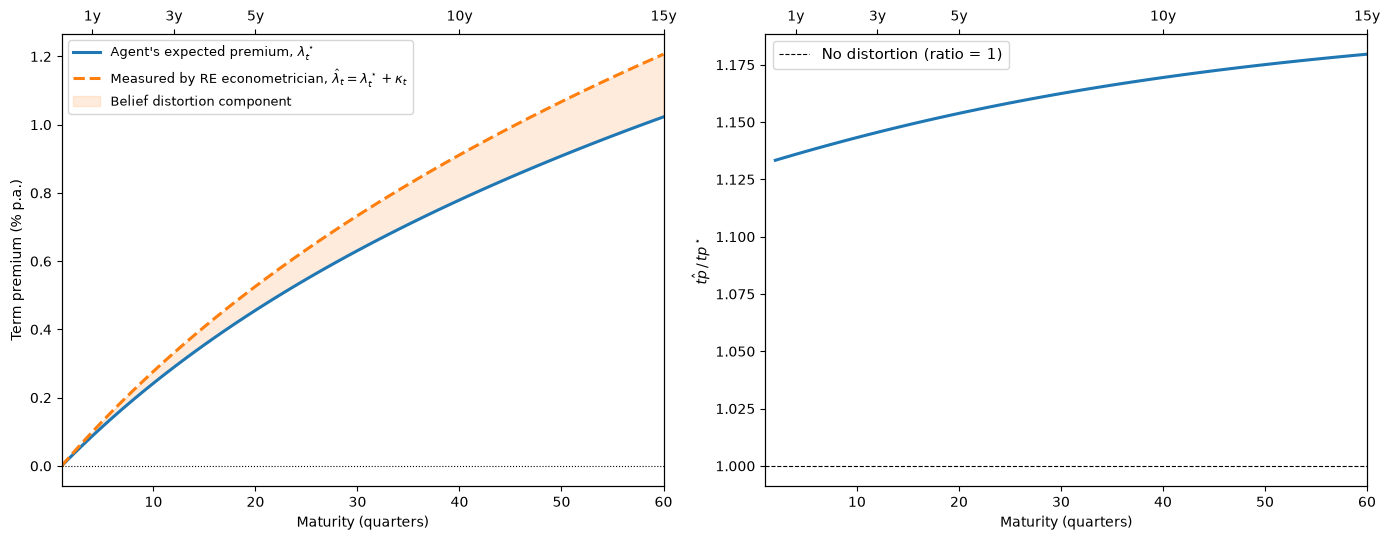
Fig. 130.5 Subjective vs. measured term premiums and overstatement ratio#
n =  4: agent 0.087%, econometrician 0.099%, ratio 1.14
n = 20: agent 0.456%, econometrician 0.526%, ratio 1.15
n = 40: agent 0.779%, econometrician 0.911%, ratio 1.17
n = 60: agent 1.023%, econometrician 1.207%, ratio 1.18
At \(z_t = 0\), the distortion is \(\kappa_t = \kappa_0 = (-0.005, 0)\), which comes from the experts’ upward bias \(\check\mu_1 = 0.005\) in forecasting the level factor.
Experts who expect higher future interest rates expect lower returns on long bonds than the returns that actually materialize on average.
The econometrician therefore overstates the term premium that the agent requires, by 14 to 18 percent in this calibration.
The persistence distortion \(\kappa_z\) makes the size and even the sign of the gap depend on the state.
for label, z in [("High rate", np.array([3.0, -2.0])),
                 ("Low rate",  np.array([-3.0, 2.0]))]:
    gap = (term_premiums(model_econ, z, n_max_db)
           - term_premiums(model_subj, z, n_max_db)) * 4 * 100
    print(f"{label}: belief-distortion gap at 5 and 15 years = "
          f"{gap[19]:.2f}%, {gap[59]:.2f}%")
High rate: belief-distortion gap at 5 and 15 years = 0.37%, 1.89%
Low rate: belief-distortion gap at 5 and 15 years = -0.23%, -1.53%
When rates are high, experts extrapolate them too far into the future, so the econometrician’s measured premium exceeds the agent’s premium by almost 2 percentage points at 15 years.
When rates are low, the gap reverses sign.
A rational-expectations econometrician therefore attributes to time-varying risk prices movements in measured excess returns that actually come from the agent’s systematic forecast errors.
Our Risk Aversion or Mistaken Beliefs? lecture explores this confounding in greater depth.
130.8. Concluding remarks#
The affine model of the stochastic discount factor provides a flexible and tractable framework for studying asset prices.
Key features are:
Analytical tractability: Bond prices are exponential affine in \(z_t\); expected returns decompose cleanly into a short rate plus a risk-price×exposure inner product.
Empirical flexibility: The free parameters \((\mu, \phi, C, \delta_0, \delta_1, \lambda_0, \lambda_z)\) can be estimated by maximum likelihood (the Kalman filter chapter describes the relevant methods) without imposing restrictions from a full general equilibrium model.
Multiple risks: The vector structure accommodates many sources of risk (monetary policy, real activity, volatility, etc.).
Belief distortions: The framework naturally accommodates non-rational beliefs via likelihood-ratio twists of the physical measure, as in Piazzesi et al. [2015].
Limits to identification: Bond prices reveal only the risk-neutral measure, so separating risk prices from belief distortions requires additional evidence, such as survey forecasts; see also The Recovery Theorem and Misspecified Recovery.
The model also connects directly to the Hansen–Jagannathan bounds studied in Doubts or Variability? and to robust control interpretations of the stochastic discount factor described in other chapters of Ljungqvist and Sargent [2018].
For finite-state approaches to asset pricing that complement the continuous-state framework here, see Asset Pricing: Finite State Models.